Abstract
The Powerful Puzzling algorithm aims to solve the problem of jigsaw puzzle solvers that work with island pieces (a group of two or more connected pieces). This is unlike current solutions that require a fully disassembled puzzle in order to work ( Citation: Abto Software, 2021, October 11 Abto Software (2021, October 11). Computer Vision Powers Automatic Jigsaw Puzzle Solver.. Retrieved from https://www.abtosoftware.com/blog/computer-vision-powers-automatic-jigsaw-puzzle-solver ) ( Citation: Terleev, 2021, October 22 Terleev, M. (2021, October 22). Jigsaw puzzle AI from A to Z. towardsdatascience. Retrieved from https://towardsdatascience.com/jigsaw-puzzle-ai-from-a-to-z-b4bdb53d8686 ) . And is a practical approach to puzzle solving that allows players the satisfaction of completing the puzzle without disassembly. The main idea behind how Powerful Puzzling works is the unrolling of border contours into a 1D strip that can be segmented up and compared with other pieces to find matches. This allows us to work in a 1 dimensional plane and not have to worry about performing brute force rotations and translations to get pieces to match ( Citation: Giorgino, T, nd Giorgino, T (nd). Computing and visualizing dynamic time warping alignments in R: The DTW package. Retrieved from https://www.jstatsoft.org/v31/i07/ ) . The Powerful Puzzling algorithm also uses Dynamic Time Warping (DTW) for both shape and color matching and combines the results to get a final match score. We found that when we apply a weighting of (2,1) for the shape and color score, respectively, we got the best performance with 3 out of the top 5 matches being correctly identified. The algorithm also introduces some high level filters that improve performance allowing the entire program to run in under 3s (1.5s for just matching).
Introduction
Jigsaw puzzles are a staple of at-home entertainment and have exploded in demand in the past year due to COVID-19 ( Citation: Miller, H, 2020, April 6 Miller, H (2020, April 6). Demand for jigsaw puzzles is surging as coronavirus keeps millions of Americans indoors. CNBC. Retrieved from https://www.cnbc.com/2020/04/03/coronavirus-sends-demand-for-jigsaw-puzzles-surging.html ) . Here we will explore the problem of an automatic jigsaw puzzle solver and present a possible solution that works under most conditions. Current solutions to the puzzle solver only work under the condition that the puzzle be fully disassembled in that each piece stands on its own, not connected to any other piece ( Citation: Abto Software, 2021, October 11 Abto Software (2021, October 11). Computer Vision Powers Automatic Jigsaw Puzzle Solver.. Retrieved from https://www.abtosoftware.com/blog/computer-vision-powers-automatic-jigsaw-puzzle-solver ) ( Citation: Terleev, 2021, October 22 Terleev, M. (2021, October 22). Jigsaw puzzle AI from A to Z. towardsdatascience. Retrieved from https://towardsdatascience.com/jigsaw-puzzle-ai-from-a-to-z-b4bdb53d8686 ) . However, this leaves out situations where there are “islands” (a connected group of two or more puzzle pieces) that requires the player to disassemble any work they have done before they can run it through the solver.
In this report we approach the problem as a tool to help players in their journey through solving a puzzle. Or in other words, we aim to provide hints as they solve the puzzle without requiring disassembly. We begin with a background on the puzzle solver and previous solutions to it, as well as any other related works. Next we explain our approach to solving the problem from a high level perspective. This is followed up with a detailed dive into how we broke up the problem into smaller subproblems and the respective solutions we came up with for those subproblems. Finally we end the report with an evaluation of the work done and a summary that includes an analysis of the results and our ideas for future work/improvements.
Background
There are many different ways one can approach the problem of the jigsaw puzzle. In our approach we take into consideration how a person might use such a tool. We don’t want to rob the player of the enjoyment of solving a puzzle and so our solution aims to solve puzzles that range from completely disassembled to partly completed with island pieces. This allows us to provide help to players at any step in their puzzle solving journey.
There already exist solutions that solve disassembled puzzles with Maxim Terleev’s article on Towards Data Science that is open source, and Abto Software’s article on their site (no source code). These solutions are relatively simple with Terleev’s being done in around 300 lines of code.
 |
 |
|---|---|
| Figure 1: Abto Software’s solver ( Citation: Abto Software, 2021, October 11 Abto Software (2021, October 11). Computer Vision Powers Automatic Jigsaw Puzzle Solver.. Retrieved from https://www.abtosoftware.com/blog/computer-vision-powers-automatic-jigsaw-puzzle-solver ) . | Figure 2: Maxim Terleev’s solver ( Citation: Terleev, 2021, October 22 Terleev, M. (2021, October 22). Jigsaw puzzle AI from A to Z. towardsdatascience. Retrieved from https://towardsdatascience.com/jigsaw-puzzle-ai-from-a-to-z-b4bdb53d8686 ) . |
Both solutions follow the same general process. Starting with image processing the goal is to extract the borders/contours of the puzzle pieces from the image. Both solutions use a simple thresholding technique to create a mask that separates the background from the pieces. Then using this mask they can extract the borders by using openCV’s findContours() function
(
Citation: OpenCV, nd
OpenCV
(nd).
Structural analysis and shape descriptors. OpenCV.
Retrieved from
https://docs.opencv.org/3.4/d3/dc0/group__imgproc__shape.html#ga95f5b48d01abc7c2e0732db24689837b
)
. With these borders they perform border segmentation to get the locks (the jigsaw nodes) on a piece that will be used for matching. For this there are two metrics to get information on how good the match is: shape matching, and color matching.
For shape matching Terleev takes a simple approach of using OpenCV’s matchShape() function with each lock. And the team at Abto Software gets a match score by getting the max of a calculation of the exclusive (XOR) of adjacent areas on the piece in place and after performing 10 pixel length translations left, right, up, and down
(
Citation: OpenCV, nd
OpenCV
(nd).
Contours : More Functions.
Retrieved from
https://docs.opencv.org/4.x/d5/d45/tutorial_py_contours_more_functions.html
)
.
Finally, for color matching Terleev uses Dynamic Time Warping (DTW) on the HSV values along each segment. And Abto samples an averaging of the four corners of each piece and uses that to compare two pieces with. Now with these metrics they can finally identify the best matches for the puzzle.
Approach
For our approach we took heavy inspiration from Terleev and followed a similar process but with a few different techniques to improve performance and include island piece matching. The approach can be summed up in 5 steps:
- image segmentation
- Border unrolling
- Lock identification
- High level filter
- Shape and color matching
Image Segmentation
Border extraction took many iterations and algorithm changes to converge to our final selected method. With each new approach, the complexity of the algorithm increased. We tried four different techniques: adaptive thresholding, clustering, superpixelization, and deep learning.
Thresholding
 |
|---|
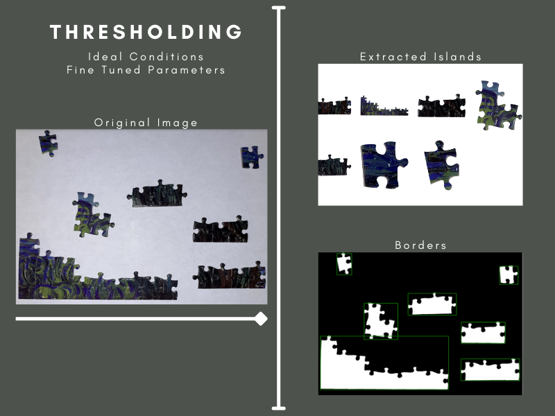
| Figure 3: Tuned thresholding segmentation in perfect conditions |
Our team started simple, with a thresholding approach. We used OpenCV’s adaptive thresholding method, which separates desirable objects in the foreground from the background using pixel intensities, followed by their find contours method to extract the island border ( Citation: SciKit-Image, nd SciKit-Image (nd). Thresholding. Thresholding - skimage v0.19.2 docs. Retrieved from https://scikit-image.org/docs/stable/auto_examples/applications/plot_thresholding.html ) . This method, although fast, was not robust enough to segment islands in any imperfect condition. Differences in lighting caused extreme fluctuations in border accuracy. Thresholding produced too many artifacts to be viable and required too much fine-tuning per image to be practical, so we decided to move on to another approach.
Clustering
 |
|---|
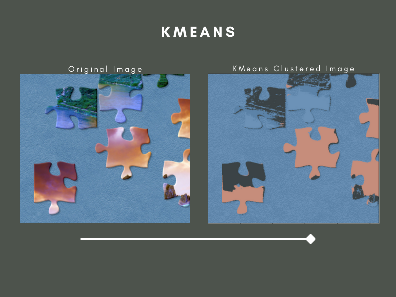
| Figure 4: Clustering using KMeans |
Our second approach was to use clustering. We tried three different methods: K-means, spectral, and fuzzy-c-means. KMeans was much slower than thresholding and provided no further advantage over it. Spectral clustering was slighter slower than KMeans and only marginally outperformed it, so we also disgraded spectral. Finally, we tried fuzzy-c clustering, which was no better or faster than KMeans. The results from our experiments suggested that clustering alone would not be able to solve this problem, so we moved on ( Citation: SciKit-Learn, nd SciKit-Learn (nd). Sklearn.cluster.kmeans. scikit.. Retrieved from https://scikit-learn.org/stable/modules/generated/sklearn.cluster.KMeans.html ) ( Citation: Scikit-Learn, nd Scikit-Learn (nd). Spectral Clustering. Retrieved from https://scikit-learn.org/stable/modules/generated/sklearn.cluster.SpectralClustering.html Citation: SciKit-Learn, nd SciKit-Learn (nd). klearn.cluster.SpectralClustering. Retrieved from https://scikit-learn.org/stable/modules/generated/sklearn.cluster.SpectralClustering.html#sklearn.cluster.SpectralClustering ) ( Citation: Scikit-Learn, nd Scikit-Learn (nd). Fuzzy C-means clustering. Fuzzy c-means clustering - skfuzzy v0.2 docs. Retrieved from https://pythonhosted.org/scikit-fuzzy/auto_examples/plot_cmeans.html ) .
Superpixelization
 |
|---|
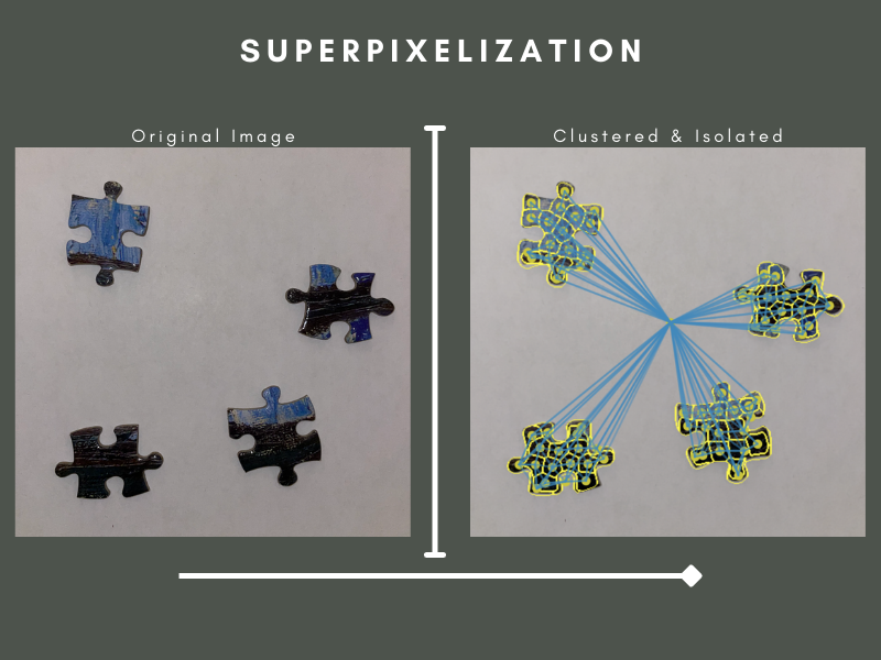
| Figure 5: Superpixelization after clustering. The resulting superpixels segment the islands |
Our third approach was to use scikit-image’s superpixelization implementation. A superpixel is a group of nearby pixels which share common characteristics like pixel intensity. Superpixelization seemed like a promising solution since it has been used in instance segmentation before, but unfortunately, it suffered from many of the same issues as thresholding. A significant problem was artifacts forming due to overlapping or missing critical superpixels. Since the islands sometimes contained complex printed patterns, the superpixels would often bleed from the island’s border to the background, ruining the edge ( Citation: SciKit Image, nd SciKit Image (nd). Comparison of segmentation and superpixel algorithms. Retrieved from https://scikit-image.org/docs/stable/auto_examples/segmentation/plot_segmentations.html ) .
However, in ideal conditions with relatively simple islands, superpixelization managed to work well. The next issue was determining the difference between a background superpixel and a foreground superpixel. Once again, we used KMeans clustering as a classifier to determine if a superpixel belongs to an island or the background. One or more sample superpixels of the background are chosen and used to determine whether or not another superpixel belongs to the background or not. The background superpixels are eliminated, leaving only those attached to islands, forming a border. Since superpixelization only worked in ideal conditions, much like thresholding, and was much slower than thresholding, we decided to move on to another approach since we could use thresholding instead of superpixelization.
Mask-RCNN
Our final approach was an image segmentation deep learning model called a Mask-RCNN built in TensorFlow ( Citation: TensorFlow, nd TensorFlow (nd). Machine Learning Framework. Retrieved from https://www.tensorflow.org/ ) . An MRCNN uses an image classification model as a backbone and convolutional layers to generate a mask of an instance. MRCNNs run in three main steps. Step one is anchor sorting and filtering. The region proposal network, a CNN that simultaneously predicts object boundaries and object scores, generates rectangular regions of interest that can potentially fully or partially contain an object. These regions of interest are then filtered down into the best contenders, yielding the anchors. In step two, the bounding boxes are refined, then in step three, the masks are generated ( Citation: He, K., Gkioxari, G., 2018, January 24 He, K., Gkioxari, G. (2018, January 24). Mask R-CNN. Retrieved from https://arxiv.org/abs/1703.06870 ) ( Citation: MatterPort, nd MatterPort (nd). [Matterport, M. (n.d.). MASK_RCNN.. Retrieved from https://github.com/matterport/Mask_RCNN/tree/master/mrcnn ) .
The challenge of this approach was the data since we had to develop most of the training instances from scratch. We hand labelled all images using the VIA image annotator to generate the data ( Citation: Dutta, A, nd Dutta, A (nd). Dutta, A. (n.d.). VGG Image annotator. Retrieved from https://www.robots.ox.ac.uk/~vgg/software/via/via_demo.html ) . Due to the unusual shapes of islands, labelling each image became a very time-consuming process. We managed to find another similar project using a MaskRCNN and a substantial number of pre-labelled pieces. Unfortunately, their project expected only a single puzzle piece per image, so all training instances were one piece, which was not as valuable for our case. Including such data in our training reduced the quality of our masks, so we decided against using them. To stretch our limited dataset as far as possible, we introduced many imgaug augmenters to our training.
Since it would be impossible to train this model from scratch with our dataset, we used transfer learning - starting from the pretrained COCO weights as a starting point ( Citation: MSCOCO, nd MSCOCO (nd). MS COCO - Common Objects In Context. Retrieved from https://cocodataset.org/#home ) . We trained for twenty epochs with a learning rate of only 0.001. After training, this technique seemed to be the most promising of all those we have tried; however, it is not without its limitations. Although it can handle segmentation in far more complex situations, it struggles with large islands. The difficulty with larger islands is due to the resolution of the masks. The masks' resolution could not be increased due to RAM limitations, but our team thinks this could have made a substantial difference in mask accuracy. With more data, we would have achieved better results for our segmentation.
 |
|---|
| Figure 6: The step by step process of the MRCNNs mask generation |
Border Unrolling:
The goal of border unrolling is to convert our 2D representation of the border (list of xy points) into a 1D representation that we can use for matching by essentially sliding across each border “strip” looking for matches. This is important for matching large islands where simple translations and rotations would not be good enough.
For this we had originally thought to follow a similar technique to Terleev’s where we “observe” the border from four sides as our 1D representation, this is illustrated below ( Citation: Terleev, nd Terleev (nd). Jigsaw puzzle geometrical fit. Simple AI. Retrieved from https://www.simple-ai.net/post/jigsaw-puzzle-geometrical-fit ) .
 |
|---|
| Figure 7: Terleev’s approach to “border unrolling” |
However, in his own words “this does not guarantee the 100% cover of the borderline”. Which is especially true for U-shaped and/or large islands. We would be losing a lot of information if we went with this method.
So, instead we choose to convert the 2D list of xy points to a 1D array by calculating the deviation angle as we move clockwise around the puzzle piece. Then we just store the deviation angles in a list as our “unrolled” border. This deviation angle is represented in the figure below as the angle between the red and blue dotted lines.
 |
|---|
| Figure 8: A visual representation of what the border unrolling algorithm extracts from the border to represent it as a 1D array. This was done using the Desmos online graphing calculator. |
The angle is found by first calculating the length of each side to the triangle formed by the three points using the euclidean distance. With this we can find the inner angle at point B by using the law of cosines then we can simply subtract by 180° (or π radians) to get the deviation angle: $$d=\pi-cos^{-1}(\frac{a^{2}+b^{2}-c^{2}}{2ab})$$
Now we need to correctly get which direction in which the angle is deviating (the sign of the angle). By the nature of arccos, if angle is greater than 90° (π/2) then the sign will flip so to stop this from happening we define an adjustment term to be the following: $$adj = \frac{\pi}{2} - d$$
And to determine if we are going left (-) or right (+) we can use the the slope of the lines AB (red line) and BC (blue line) with the adjustment term to get the following equation: $$s = sign(\frac{m_1 - m_2}{1 + m_1*m_2} * adj)$$
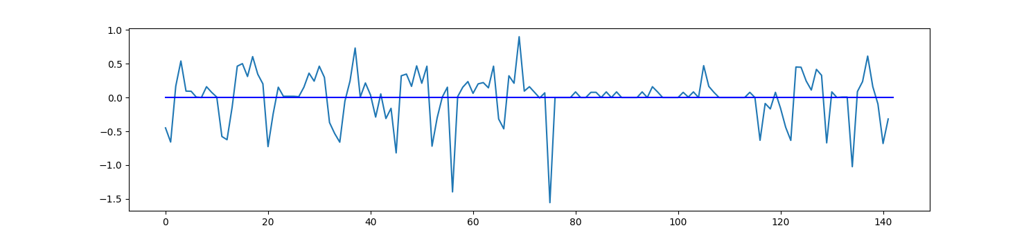
And by multiplying d with s we get our final angle that includes the direction of the deviation. One important thing to note is that we can’t sample every three points to get our angles otherwise our unrolled border would be made up of mostly zero degree angles and noise would have a much larger impact (see figure 9). So, to solve this we make sure to pick points that are 25 positions away from each other.
 |
|---|
 |
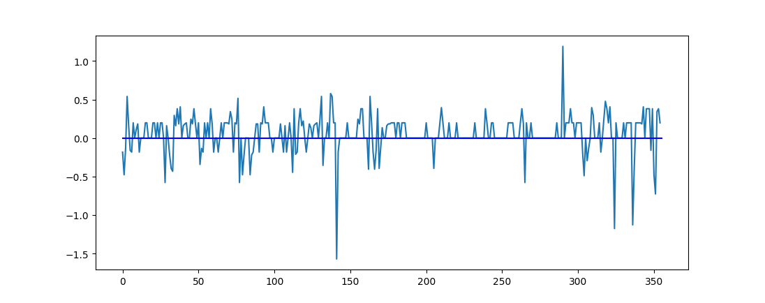 |
| Figure 9: Plots showing what the unrolling algorithm does to the border. Top: the original border. Middle: the unrolled border with a sampling rate of 25. Bottom: the unrolled border with a sampling rate of 10. |
Lock Identification:
The lock of a puzzle piece is its jigsaw segments that form the connections with other pieces. We need to be able to smartly find these locks no matter how many there are on the island using the unrolled border from the previous step.
This is done by iterating through the unrolled border and classifying points as “line points” and “non-line points” depending on if they are within a certain threshold. The threshold determines if they are close enough to 0 to be considered as a straight line (essentially zero deviation angle).
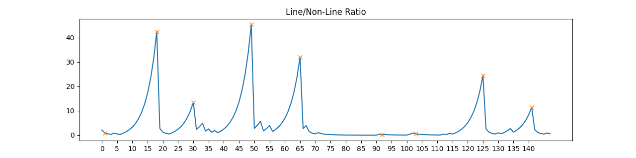
And as we are iterating through the unrolled border and classifying points we also keep track of the ratio of line points to non-line points at each iteration. The ratio also includes a $\gamma$ forgetting factor so that as we travel along the unrolled border points that are further away don’t impact the ratio as much. In other words the lower the $\gamma$ the less we care about previous points. The formula for this ratio is as follows, where $N$ and $M$ are the number of line and non-line points respectively. $$ratio = \frac{L_{new} + L_{old}*\gamma}{N_{new} + N_{old}*\gamma}$$
Iterating through the entire border we get the following plot for the ratios where it becomes immediately clear where the locks/jigsaw nodes are.
 |
|---|
Figure 10: a plot of the ratios of line points to non-line points with x markers for the peaks that are identified by SciPy’s find_peaks_cwt() function
(
Citation: SciPy, nd
SciPy
(nd).
Scipy.signal.find_peaks_cwt. scipy.signal.find_peaks_cwt - SciPy v1.8.0 Manual.
Retrieved from
https://docs.scipy.org/doc/scipy/reference/generated/scipy.signal.find_peaks_cwt.html
)
. |
Note how the peaks in the figure above all match up with the locations of the tips of locks on the original border. Also note that there is a peak for the node that is at the end of the unrolled border array (this is done by continuing the ratio for 10 more points from the start). And so using SciPy’s find_peaks_cwt() we can quickly target these nodes and make cuts to the left and right of the peak where we encounter a line-point again. And with some extra padding we have successfully identified the locks:
 |
|---|
| Figure 11: GIF illustrating the entire lock identification process. Red and yellow points indicate the “line” and “non-line” points of the border. Lock segments are highlighted in green with a red + sign indicating its start, and a blue X indicating where it ends. |
High level filter
Taking a look back at the final result from lock identification we note that some segments are not actually locks and are just straight line segments detected due to random noise. So, here we will filter out these unwanted segments and also classify locks as concave (into the island) or convex (sticking out of the island). This will improve performance by only focusing on probable matches (convex locks matching with concave locks).
Starting with the first filter we can identify line segments by performing a linear regression (on the original xy border values) and returning the Mean Squared Error of the regression. This MSE will be low for line segments (0.0 up to 2.0) and large to extremely large for any segment with curves on it (300 up to 1500). So by using a threshold of 5.0 we can easily filter out straight line segments. However, one limitation to this is that we have to perform regression twice, alternating which axis is the horizontal axis to prevent vertical line segments from resulting in a much higher MSE due to its near infinite slope.
Finally, for our second filter we can identify concave from convex locks by fitting a 2nd degree polynomial on the unrolled border using Numpy’s polyfit() function
(
Citation: Numpy, nd
Numpy
(nd).
Numpy.polyfit. numpy.polyfit.
Retrieved from
https://numpy.org/doc/stable/reference/generated/numpy.polyfit.html
)
. Then we can simply take the sign of the coefficient for the highest power as a high level indication of its lock shape (negative for convex, positive for concave). Now we can check to see if a pair of segments are shape compatible before diving into the more computationally expensive shape and color matching.
Shape and color matching
Shape matching
For shape matching we originally tried to use OpenCV’s matchShape() function with the original xy border contours. This would calculate Hu moments for each segment pair, and the segment pair with the lowest Hu moment would be the best match
(
Citation: OpenCV, nd
OpenCV
(nd).
Contours : More Functions.
Retrieved from
https://docs.opencv.org/4.x/d5/d45/tutorial_py_contours_more_functions.html
)
. However, this failed due to the curved nature of each segment and how unevenly distributed the points were (densest around curved sections).
So instead, we chose to use Dynamic Time Warping (DTW) with the unrolled borders that we had segmented earlier. DTW is a popular technique commonly used for comparing timeseries-like data to get a distance measure and local stretch or compressions that can be applied to the timeseries to map them on top of each other
(
Citation: Giorgino, T, nd
Giorgino, T
(nd).
Computing and visualizing dynamic time warping alignments in R: The DTW package.
Retrieved from
https://www.jstatsoft.org/v31/i07/
)
. This makes DTW an almost perfect candidate for comparing two unrolled border segments. In Tarleev’s approach they use an approximate DTW algorithm from the fastDTW python package for color matching
(
Citation: Salvador & Chan, 2021, October
Salvador,
S. & Chan,
P.
(2021, October).
FastDTW: Toward Accurate Dynamic Time Warping in Linear Time and Space.
Retrieved from
https://cs.fit.edu/~pkc/papers/tdm04.pdf
)
(
Citation: Terleev, 2021, October 22
Terleev,
M.
(2021, October 22).
Jigsaw puzzle AI from A to Z.
towardsdatascience. Retrieved from
https://towardsdatascience.com/jigsaw-puzzle-ai-from-a-to-z-b4bdb53d8686
)
. However, in this case where we have a short series length and a narrow warping factor (how much the pieces need to warp to overlay) we decided against fastDTW in favor of the standard dtw-python package. This is supported by how in our specific case FastDTW is generally slower despite being an approximation
(
Citation: Wu, R., & Keogh, E. J., 2021, August 26
Wu, R., & Keogh, E. J.
(2021, August 26).
FASTDTW is approximate and generally slower than the algorithm it approximates.
Retrieved from
https://arxiv.org/abs/2003.11246
)
.
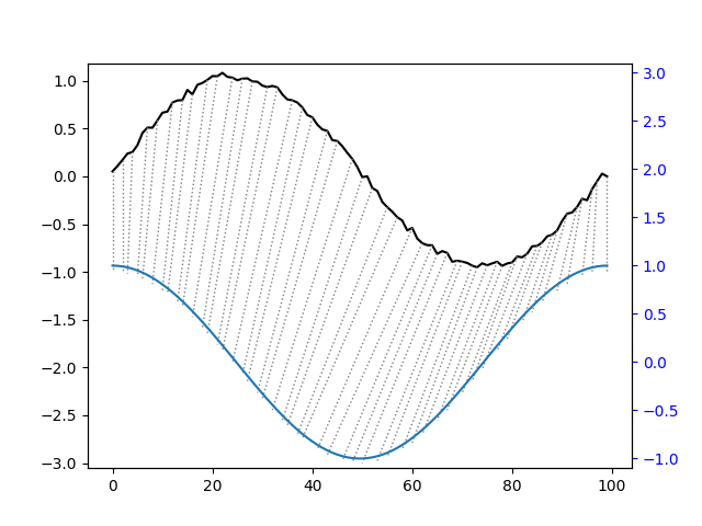 |
|---|
| Figure 12: Visualization of how DTW works for when comparing a segment of the sine and cosine graphs. |
So, DTW was performed on lock segments of the 1D unrolled border for shape matching. This would tell us crucial information about how well two locks match up with each other without needing to translate it around for a more accurate measure.
Color matching
For color matching, a bit more work was required to get a proper measure of how similar the two colors are. The first of which was to get the right sample of xy-coordinates that are guaranteed to be within the puzzle piece. This required iterating through the lock segment’s xy points on the original image and calculating orthogonal points to the border on the puzzle piece. This ensures that the sampled points we use are not part of the background. We also need to apply a median blur to the image to reduce the impact of noise.
This calculation, like with border unrolling, requires sampling points. Here we only need two points where we treat the line connecting them as the hypotenuse to a right angled triangle. Then we can calculate all the length of all the sides of the triangle and use that to calculate the position of the orthogonal point with the following equations: $$c_x = A_x-d_{ist}*\frac{h}{H}$$ $$c_y = A_y+d_{ist}*\frac{w}{H}$$
Where $c$ is the orthogonal point, $d_{ist}$ is the distance away from the border, and $h, w,$ and $H$ are the height, width, and hypotenuse of the right triangle formed by the sampled points A and B respectively (illustrated in the figure below).
 |
|---|
| Figure 13: a GIF, created using Desmos, illustrating how two sampled points from the border (points A and B) can be used to find a third point (c) that is orthogonal from the border and at a fixed distance $d_{ist}$. |
With this we can now sample points that are a better representation of what the colors at a border segment really are like. This now allows us to perform our final matching using DTW and the HSV values from the sampled points along the lock segments. For this we will need to use a multi-dimensional version of DTW to account for the 3 channels in each HSV point. We chose to use DTWi as it was the simplest and more efficient method. With DTWi we simply treat each channel as its own time series and perform normal DTW, then we get the cumulative value across all the channels to be our final distance score ( Citation: Shokoohi-Yekta & Hu, 2016, February 15 Shokoohi-Yekta, M. & Hu, B. (2016, February 15). Generalizing DTW to the multi-dimensional case requires an adaptive approach - data mining and knowledge discovery. Retrieved from https://link.springer.com/article/10.1007/s10618-016-0455-0 ) .
Putting it all together
Now that we have a way to measure the color and shape distance of two segments we can take their normalized score and combine them in a weighted sum for our final distance/match score. The weighted sum allows us to favor one score over the other, depending on which is a better metric for match compatibility.
Evaluation
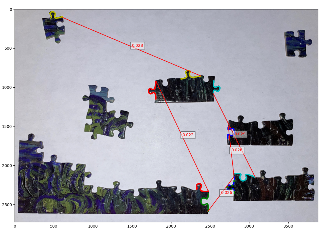
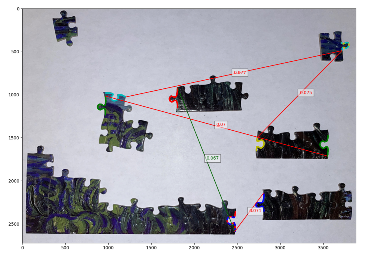
Starting with the final product (figure 14) we can see that the Powerful Puzzling algorithm that we have developed successfully identifies 3 connections out of the top 5 matches when we apply the right weighting to the match scores.
 |
|---|
 |
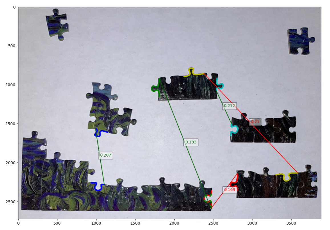 |
| Figure 14: The final output of the Powerful Puzzling algorithm under different score weightings for shape and color. Here we can see the top 5 matches it found along with their match score (the lower the better). lines in green indicate correctly identified matches. Top: a weighting of (0,1) for shape and color respectively. Middle: a weighting of (1,0). Bottom: a weighting of (2,1). |
And in terms of performance the matching algorithm performs exceptionally well taking an overall time <2s to run. The main bottleneck being the actual extraction of the border contours themselves.
Table 1: The time it takes for each step of the powerful puzzling algorithm in seconds. For image segmentation we show both MRCNN and thresholding techniques (of which MRCNN takes advantage of GPU acceleration by running on Google Colab)
| Steps | Trial 1 | Trial 2 | Trial 3 | Average |
|---|---|---|---|---|
| Image Segmentation (Thresholding) | 1.312 | 1.308 | 1.312 | 1.311 |
| Image Segmentation (MRCNN, Colab) | 0.412 | 0.392 | 0.419 | 0.407 |
| Border Unrolling and Lock Identification | 0.610 | 0.614 | 0.610 | 0.611 |
| Filtering and Matching | 0.861 | 0.861 | 0.849 | 0.857 |
| Total | 2.783 | 2.783 | 2.771 | 2.779 |
Summary
Based on the results from evaluation we believe the Powerful Puzzling algorithm performed as we expected. It manages to be a successful tool for players as even if there are some incorrect match ups those can be easily ruled out by the player. And when taking a look at incorrect matches we can see that it isn’t a total catastrophic failure (e.g. matching with a line segment, or matching two completely incompatible shapes) with some pieces that arguably could match.
We believe the main culprit for the majority of the failed matches is due to how noisy color matching is. This is evident when we compare the results of matches from the different weightings. We can see that with only shape matching (middle plot in figure 14) we still manage to get at least one match, but on the other hand using only color matching (top plot in figure 14) gets us no correct matches. One way to overcome the noisiness of color matching would be to take an averaging of pixels along the orthogonal line to the border instead of a single pixel. Nonetheless we know that color matching is still effective by how much better the performance is when we have a weighting of (2,1) compared to just shape matching alone (bottom plot in figure 15).
Aside from improving the color matcher, another addition we feel would improve the accuracy of the matcher is to prevent duplicate matches with a single segment from occurring. This means for any segment where we have two pieces that are contested on a single segment (e.g. the red and green segment in the bottom plot of figure 14) the match with the lower score would be forced to pick its next best candidate instead. This would be a difficult problem to solve as we would need to keep track of all the previous segments that each segment matches with and continuously check if they have been overtaken by a better match to pick the next candidate. This would also need to work in reverse to restore segments when a match that overtook a previous match is overtaken on its other segment.
We also feel that we could reduce the noise by improving the border extraction process during image segmentation. It would be compelling to increase the resolution of the mask, which we could not do in our project due to RAM limitations. Increasing the masks' resolution would result in more accurate masks and allow for large islands to be more accurately segmented. It would also be interesting to train on more data. Only one of our group members worked on compiling and labeling the dataset, which was a long process. If more people contributed to building a dataset, we could see better results.
Another idea we would like to have explored is using a mix of thresholding or grab cut (like seen in photoshop selecting) and Mask RCNN, where this technique would use the non-deep learning techniques on the large islands ( Citation: OpenCV, nd OpenCV (nd). Interactive Foreground Extraction using GrabCut Algorithm. Retrieved from https://docs.opencv.org/3.4/d8/d83/tutorial_py_grabcut.html ) . Combining these two methods could solve the two most significant problems we encountered. The Mask RCNN works exceptionally well for single pieces, even in a noisy background, while thresholding works very poorly with a noisy background. A limitation of the grab cut method is that a region of interest must be defined to segment; however, if we combined grab cut with the Mask RCNN, which produces regions of interest within their bounding boxes, this limitation can be overcome.
To conclude, the work we have done here is relatively still in its infancy, there are no readily available papers that discuss solutions for jigsaw puzzle solvers that work with island pieces. We believe that there is still a lot that can be improved with our Powerful Puzzling algorithm. And with this paper we wish to introduce this concept of a puzzle solver that can work for islands to more people in the field which hopefully leads to an improved version of the Powerful Puzzling algorithm with a higher matching accuracy.
References
- Abto Software (2021, October 11)
- Abto Software (2021, October 11). Computer Vision Powers Automatic Jigsaw Puzzle Solver.. Retrieved from https://www.abtosoftware.com/blog/computer-vision-powers-automatic-jigsaw-puzzle-solver
- Miller, H (2020, April 6)
- Miller, H (2020, April 6). Demand for jigsaw puzzles is surging as coronavirus keeps millions of Americans indoors. CNBC. Retrieved from https://www.cnbc.com/2020/04/03/coronavirus-sends-demand-for-jigsaw-puzzles-surging.html
- Giorgino, T (nd)
- Giorgino, T (nd). Computing and visualizing dynamic time warping alignments in R: The DTW package. Retrieved from https://www.jstatsoft.org/v31/i07/
- Salvador & Chan (2021, October)
- Salvador, S. & Chan, P. (2021, October). FastDTW: Toward Accurate Dynamic Time Warping in Linear Time and Space. Retrieved from https://cs.fit.edu/~pkc/papers/tdm04.pdf
- Wu, R., & Keogh, E. J. (2021, August 26)
- Wu, R., & Keogh, E. J. (2021, August 26). FASTDTW is approximate and generally slower than the algorithm it approximates. Retrieved from https://arxiv.org/abs/2003.11246
- He, K., Gkioxari, G. (2018, January 24)
- He, K., Gkioxari, G. (2018, January 24). Mask R-CNN. Retrieved from https://arxiv.org/abs/1703.06870
- MatterPort (nd)
- MatterPort (nd). [Matterport, M. (n.d.). MASK_RCNN.. Retrieved from https://github.com/matterport/Mask_RCNN/tree/master/mrcnn
- TensorFlow (nd)
- TensorFlow (nd). Machine Learning Framework. Retrieved from https://www.tensorflow.org/
- Dutta, A (nd)
- Dutta, A (nd). Dutta, A. (n.d.). VGG Image annotator. Retrieved from https://www.robots.ox.ac.uk/~vgg/software/via/via_demo.html
- MSCOCO (nd)
- MSCOCO (nd). MS COCO - Common Objects In Context. Retrieved from https://cocodataset.org/#home
- OpenCV (nd)
- OpenCV (nd). Structural analysis and shape descriptors. OpenCV. Retrieved from https://docs.opencv.org/3.4/d3/dc0/group__imgproc__shape.html#ga95f5b48d01abc7c2e0732db24689837b
- SciPy (nd)
- SciPy (nd). Scipy.signal.find_peaks_cwt. scipy.signal.find_peaks_cwt - SciPy v1.8.0 Manual. Retrieved from https://docs.scipy.org/doc/scipy/reference/generated/scipy.signal.find_peaks_cwt.html
- Scikit-Learn (nd)
- Scikit-Learn (nd). Fuzzy C-means clustering. Fuzzy c-means clustering - skfuzzy v0.2 docs. Retrieved from https://pythonhosted.org/scikit-fuzzy/auto_examples/plot_cmeans.html
- OpenCV (nd)
- OpenCV (nd). Interactive Foreground Extraction using GrabCut Algorithm. Retrieved from https://docs.opencv.org/3.4/d8/d83/tutorial_py_grabcut.html
- SciKit-Learn (nd)
- SciKit-Learn (nd). Sklearn.cluster.kmeans. scikit.. Retrieved from https://scikit-learn.org/stable/modules/generated/sklearn.cluster.KMeans.html
- OpenCV (nd)
- OpenCV (nd). Contours : More Functions. Retrieved from https://docs.opencv.org/4.x/d5/d45/tutorial_py_contours_more_functions.html
- Shokoohi-Yekta & Hu (2016, February 15)
- Shokoohi-Yekta, M. & Hu, B. (2016, February 15). Generalizing DTW to the multi-dimensional case requires an adaptive approach - data mining and knowledge discovery. Retrieved from https://link.springer.com/article/10.1007/s10618-016-0455-0
- Numpy (nd)
- Numpy (nd). Numpy.polyfit. numpy.polyfit. Retrieved from https://numpy.org/doc/stable/reference/generated/numpy.polyfit.html
- Terleev (nd)
- Terleev (nd). Jigsaw puzzle geometrical fit. Simple AI. Retrieved from https://www.simple-ai.net/post/jigsaw-puzzle-geometrical-fit
- SciKit-Learn (nd)
- SciKit-Learn (nd). klearn.cluster.SpectralClustering. Retrieved from https://scikit-learn.org/stable/modules/generated/sklearn.cluster.SpectralClustering.html#sklearn.cluster.SpectralClustering
- SciKit Image (nd)
- SciKit Image (nd). Comparison of segmentation and superpixel algorithms. Retrieved from https://scikit-image.org/docs/stable/auto_examples/segmentation/plot_segmentations.html
- SciKit-Image (nd)
- SciKit-Image (nd). Thresholding. Thresholding - skimage v0.19.2 docs. Retrieved from https://scikit-image.org/docs/stable/auto_examples/applications/plot_thresholding.html
- Terleev (2021, October 22)
- Terleev, M. (2021, October 22). Jigsaw puzzle AI from A to Z. towardsdatascience. Retrieved from https://towardsdatascience.com/jigsaw-puzzle-ai-from-a-to-z-b4bdb53d8686