LOCM Action Model Acquisition

Introduction

Model acquisition is a subfield of automated planning with the goal of learning action models from state traces– a sequence of executed actions. An action model represents an action and its effect on the state, including its preconditions and add effects. The sequence either terminates at a goal state or includes enough actions to capture the search space. These traces are used to reverse engineer the domain files which accurately capture the problem setting.

LOCM is a model acquisition algorithm– the foundational paper of the LOCM suite ( Citation: Cresswell, McCluskey & al., 2013 Cresswell, S., McCluskey, T. & West, M. (2013). Acquiring planning domain models using LOCM. Knowledge Engineering Review. Retrieved from http://eprints.hud.ac.uk/id/eprint/9052/1/LOCM_KER_author_version.pdf ) . LOCM generates Planning Domain Definition Language (PDDL) files as output by defining object (sort) centered finite state machines (FSMs) which track the state of the objects found in the trace. The FSMs model the interactions between objects after they undergo state transitions carried out by an ordered list of relevant actions pertaining to each sort.

The algorithm was implemented into the MACQ library ( Citation: Callanan, De Venezia & al., 2022 Callanan, E., De Venezia, R., Armstrong, V., Paredes, A., Chakraborti, T. & Muise, C. (2022). MACQ: A Holistic View of Model Acquisition Techniques. ICAPS Workshop on Knowledge Engineering for Planning and Scheduling (KEPS). Retrieved from https://arxiv.org/abs/2206.06530 ) , written in python. The library provides methods to import and represent PDDL problems, with methods to extract and generate example traces.

Background

We worked on implementing LOCM ( Citation: Cresswell, McCluskey & al., 2013 Cresswell, S., McCluskey, T. & West, M. (2013). Acquiring planning domain models using LOCM. Knowledge Engineering Review. Retrieved from http://eprints.hud.ac.uk/id/eprint/9052/1/LOCM_KER_author_version.pdf ) and LOCM2 ( Citation: Cresswell & Gregory, 2011 Cresswell, S. & Gregory, P. (2011). Generalised Domain Model Acquisiton from Action Traces. Proceedings of the Twenty-First International Conference on Automated Planning and Scheduling . Retrieved from https://ojs.aaai.org/index.php/ICAPS/article/view/13476/13325 ) . The authors’s LOCM implementation was written in prolog, however no implementation using a well documented, modern library such as MACQ exists currently.

The paper builds upon assumptions and hypotheses of the underlying state trace data to develop a working model acquisition algorithm. The entire algorithm runs only off of the sequential list of actions taken in a plan. Action objects hold only their parity and which objects (sorts) are used as arguments. These ‘lifted' arguments generalize our algorithm, since we are more interested in the fact that a truck can drive rather than which truck drives. To rephrase, we are only concerned with general object behaviour.

PDDL is a language which, at a high level, allows users to describe their problem setting with code. Automated planning is used to power some of mankind’s most ambitious projects, like the Mars Perseverance Rover from JPL (NASA) ( Citation: Bhaskaran, Agrawal & al., 2020 Bhaskaran, S., Agrawal, J., Chien, S. & Chi, W. (2020). Using a Model of Scheduler Runtime to Improve the Effectiveness of Scheduling Embedded in Execution. ICAPS Workshop on Planning and Robotics (PlanRob). Retrieved from https://ai.jpl.nasa.gov/public/documents/papers/Using_a_model_ICAPS2020_WS.pdf ) and IBM Watson ( Citation: IBM Watson, nd IBM Watson (nd). AI Planning Publications. Retrieved from https://researcher.watson.ibm.com/researcher/view_group_pubs.php?grp=8432 ) . Planning solvers use the domain files as well as the relevant problem instance to try to find actions which result in a predefined goal state.

LOCM

At a high level LOCM is an action model acquisition technique, based on constructing object-sort centric FSM. It receives a single action sequence as input, including only the name of the action taken each step and the list of affected object names. LOCM assumes no prior knowledge of the planning domain theory, i.e. that no information is given about the state in each step, the predicates, the real object sorts, the action models, the initial state, or the goal. There is also no knowledge or assumptions about the rationality of the agent that produced the input action sequence. The technique extracts the action models from the FSMs it constructs, learning lifted action models.

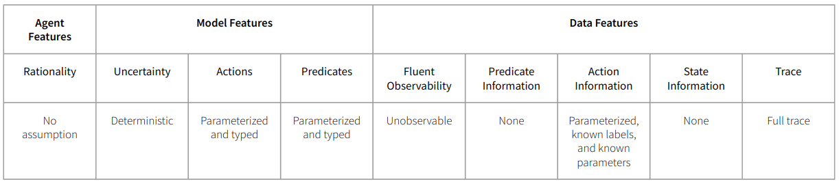
Therefore, LOCM can be characterized in the MACQ acquisition technique taxonomy as: making no assumption about the agent’s rationality; learning a deterministic, parameterized and typed model; and operating on a single full trace with complete (parameterized and labeled) action information, but no predicate, state, or fluent information.

The algorithm first extracts the unique object sorts in the domain (i.e. the ostensibly distinct types of objects), and partitions the trace into consecutive actions for each object. This is used to build the FSMs for each sort, and then the later steps augment these FSMs with parameters and filter them to get as accurate of a model as possible of the associations between the objects. Finally, the augmented and filtered FSMs are used to derive the action models and output as PDDL

LOCM

LOCM is composed of seven main steps, plus the prerequisite extraction of the object sorts.

Sort Formation

Formation of the sorts is based on the first two assumptions. The first assumption, “Structure of the Universe”, states that the universe of objects can be divided into disjoint subsets (sorts) where objects of the same sort are affected in the same way by actions and can be described by the same set of states. The second assumption, “Consistency of Action Format”, formally describes how the sorts can be extracted from the action sequence. It states that any two objects that occupy the same argument position in a given action must share the same sort.

Despite the relatively straightforward reasoning used to derive sorts, no actual algorithm was given for this and designing our own was non-trivial. After some deliberation and failed implementation attempts with other data structures, we settled on representing the sorts as a list of sets (sorts) containing the objects belonging to that sort, and an accompanying hashmap to map actions and their parameters to the assigned sort-set index. We found that other representations required complex recursive functions to update the sorts as we iterated over the action sequence, but using this representation allows the update to happen in a single pass.

The simplest cases are when it is the first occurrence of the action. If the object under consideration is not yet sorted we can just add a new set to our list, containing only the current object, and record the sort the action parameter belongs to.

# instantiate new list tracking the sorts of the action's parameters
ap_sort_pointers[action.name] = []

# for each parameter of the action
for obj in action.obj_params:
    if obj.name not in sorted_objs:  # unsorted object
            # append a sort (set) containing the object
            sorts.append({obj})

            # record the object has been sorted and the index of the sort it belongs to
            sorted_objs.append(obj.name)
            obj_sort = len(sorts) - 1
            ap_sort_pointers[action.name].append(obj_sort)

If the object has seen before, then we just need to record the sort for the action parameter.

# in same loop as above
    else: # object already has a sort
        obj_sort = get_obj_sort(obj) # look up the sort of the object
        ap_sort_pointers[action.name].append(obj_sort)

When we’ve seen the action before and assigned sorts for each of its parameters, we have to make sure the objects in this new occurrence are sorted accordingly. This is trivial when the objects haven’t been previously seen and assigned a sort, as we track the sort associated with each actions' parameters so the objects can simply be added to the correct set.

for ap_sort, obj in zip(
    ap_sort_pointers[action.name], action.obj_params
    ):
  if obj.name not in sorted_objs:  # unsorted object
# add the object to the sort of current action parameter
  sorts[ap_sort].add(obj)
sorted_objs.append(obj.name)

However, if the object has already been assigned a sort and it does not match the sort for the action’s previous parameters, then we must merge the two sets. This invalidates any action parameter pointers pointing to either of these two sorts, so we must go update those afterward.

# retrieve the sort the object belongs to
obj_sort = get_obj_sort(obj)

# check if the object's sort matches the action paremeter's
# if so, do nothing and move on to next step
# otherwise, unite the two sorts
if obj_sort != ap_sort:
    # unite the action parameter's sort and the object's sort
    sorts[obj_sort] = sorts[obj_sort].union(sorts[ap_sort])

    # drop the not unionized sort
    sorts.pop(ap_sort)

    old_obj_sort = obj_sort
    obj_sort = get_obj_sort(obj)

    min_idx = min(ap_sort, obj_sort)

    # update all outdated records of which sort the affected objects belong to
    for action_name, ap_sorts in ap_sort_pointers.items():
        for p, sort in enumerate(ap_sorts):
            if sort == ap_sort or sort == old_obj_sort:
                ap_sort_pointers[action_name][p] = obj_sort
            elif sort > min_idx:
                ap_sort_pointers[action_name][p] -= 1

Step 1: Induction of Finite State Machines

The first listed step of the algorithm builds the FSMs for each sort based on three formal assumptions (3-5 in the paper). “States of a Sort” asserts that each action causes every object it acts on to undergo some transition. The transition action $A_i$ causes for the object occupying its $k^{th}$ parameter is labeled $A_i.k$. Each transition $A_i.k$ moves the object occupying the $k^{th}$ action parameter from some start state $start(A_i.k)$ to an end state $end(A_i.k)$, which may be identical to the start state (i.e. the transition does not cause the object to change states). Each $A_i.k$ forms a transition in the FSMs. The other two assumptions, “Continuity of Object Transitions” and “Transitions are 1-1”, formally state the logic used to combine identical transitions to build coherent state machines. Continuity tells us that two consecutive actions on an object must share a state, i.e. the latter transition starts in the end state of the prior. Formally, if the $i^{th}$ and $j^{th}$ actions are consecutive for some object, and both objects appear in the same position in the action ($O=O_{i,k}=O_{j,l}$), then $end(A_i.k)=start(A_j.l)$. These transitions should also be considered as consecutive for the sort the object belongs to when building the state machine. Transitions being 1-1 quite simply means that same actions share start and end states. Formally, if $A_i = A_j$, then $start(A_i.k) = start(A_j.k)$ and $end(A_i.k) = end(A_j.k)$.

A pseudocode algorithm was provided for this step, though it still left a lot of room for interpretation in the actual implementation.

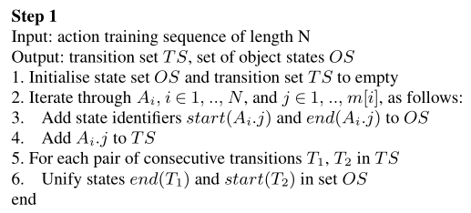
As with sort formation, a lot of time was spent figuring out what data structures could best represent the various objects and collections in the algorithm to balance efficiency and how directly we could follow the pseudocode. The main things we need to represent are the transitions $A.P$, the transition set $TS$, and the set of unique object states $OS$. In $OS$, we again represent unique states in a list of sets to enable straightforward merging of identical states, and as such need an auxiliary hashmap to track pointers mapping $A.P$s to their start and end states.

@dataclass
class AP:
    """Action.Position (of object parameter). Position is 1-indexed."""

    action: Action
    pos: int  # NOTE: 1-indexed
    sort: int

    def __repr__(self) -> str:
        return f"{self.action.name}.{self.pos}"

    def __hash__(self):
        return hash(self.action.name + str(self.pos))

    def __eq__(self, other):
        return hash(self) == hash(other)


class StatePointers(NamedTuple):
    start: int
    end: int

    def __repr__(self) -> str:
        return f"({self.start} -> {self.end})"


Sorts = Dict[str, int]  # {obj_name: sort}
APStatePointers = Dict[int, Dict[AP, StatePointers]]  # {sort: {AP: APStates}}


OSType = Dict[int, List[Set[int]]]  # {sort: [{states}]}
TSType = Dict[int, Dict[PlanningObject, List[AP]]]  # {sort: {obj: [AP]}}


...


# initialize the state set OS and transition set TS
OS: OSType = defaultdict(list)
TS: TSType = defaultdict(dict)

# track pointers mapping A.P to its start and end states
ap_state_pointers = defaultdict(dict)

In the algorithm, the first step (1) is covered by the initialization shown above. The second step (2), iterating over the action sequence for each object, requires first partitioning the action sequence accordingly.

# collect action sequences for each object
obj_traces: Dict[PlanningObject, List[AP]] = defaultdict(list)
for obs in obs_trace:
    action = obs.action
    if action is not None:
        # add the step for the zero-object
        obj_traces[zero_obj].append(AP(action, pos=0, sort=0))
        # for each combination of action name A and argument pos P
        for j, obj in enumerate(action.obj_params):
            # create transition A.P
            ap = AP(action, pos=j + 1, sort=sorts[obj.name])
            obj_traces[obj].append(ap)

This allows us to loop over the objects and their consecutive sequences, and the remaining parts of the algorithm can all happen in this loop. For each transition $A.P$ in an object’s sequence we add $A_i.j$ to $TS$ (4), and then check if it is the first occurrence of the transition for the sort. If it is, we add new unique states for $start(A.P)$ and $end(A.P)$ and initialise its state pointers (3). Then we check if any unification needs to take place (5). To do this, we track the pointer to the previous end state, and check if it points to the same state as the current start state, and if not combine the state-sets.

# iterate over each object and its action sequence
for obj, seq in obj_traces.items():
    state_n = 1  # count current (new) state id
    sort = sorts[obj.name] if obj != zero_obj else 0
    TS[sort][obj] = seq  # add the sequence to the transition set
    prev_states: StatePointers = None  # type: ignore
    # iterate over each transition A.P in the sequence
    for ap in seq:
        # if the transition has not been seen before for the current sort
        if ap not in ap_state_pointers[sort]:
            ap_state_pointers[sort][ap] = StatePointers(state_n, state_n + 1)

            # add the start and end states to the state set as unique states
            OS[sort].append({state_n})
            OS[sort].append({state_n + 1})

            state_n += 2

        ap_states = ap_state_pointers[sort][ap]

        if prev_states is not None:
            # get the state ids (indecies) of the state sets containing
            # start(A.P) and the end state of the previous transition
            start_state, prev_end_state = LOCM._pointer_to_set(
                OS[sort], ap_states.start, prev_states.end
            )

            # if not the same state set, merge the two
            if start_state != prev_end_state:
                OS[sort][start_state] = OS[sort][start_state].union(
                    OS[sort][prev_end_state]
                )
                OS[sort].pop(prev_end_state)

        prev_states = ap_states

Step 2: Zero analysis

Zero analysis catches the behaviour of implicitly defined objects in the trace. For instance, in a card game, one can only do the action of picking up a card after putting down a card and vice versa. The back and forth nature of this action means there is an implicitly defined ‘hand' object which tracks what action can come next, but this would be otherwise missed in step 1. Zero analysis follows the same procedure as step 1 and, as seen in the code snippets above, we incorporated it into the step. This avoids having to run the exact same loop twice. At the end of the step, if the resulting state machine has only one state it is removed; Otherwise implicit behaviour has been detected.

Step 3: Induction of Parameterised FSMs

Step 1 of LOCM created the FSMs for each sort found, but they currently only capture state information of objects within the sort. To capture the relationships between objects of different sorts, we need to parameterize the states. To accomplish this, step 3 forms hypotheses about the state parameters, and then tests them against the consecutive action sequences, removing hypotheses as contradictions arise. This is based on Hypothesis 3, “Parameter Association”, which states that if two consecutive transitions share a parameter of another (same) sort, hypothesise that their shared state (end of the prior, start of the latter) has a parametric association of that other sort. These hypotheses are then filtered by checking all pairs of consecutive actions and confirming it is always the same object in the hypothesised parameter position.

A pseudocode algorithm was also provided for this step, breaking it into two distinct parts: forming the hypotheses, and testing and filtering them against the consecutive sequences.

This introduces another collection needing representation, the hypothesis set $HS$, and the component hypotheses $H=\langle S, B, k, k', C, l, l', G, G' \rangle$, where $S$ is the state, $B$ is the incoming action, $k$ is the position of the main object of consideration in $B$, $k'$ is the position of the potential parameter object in $B$, $C$, $l$ and $l'$ are the same for the outgoing action, $G$ is the sort of the main object, and $G'$ is the sort of the potential parameter. To perform the checks efficiently, we noticed that matching is done on a subset of $H$: $\langle B, k, C, l \rangle$, and so we employed a custom representation for the step. We used a hashmap for $HS$, with $\langle B, k, C, l \rangle$ as the key and the set of associated $\langle S, k', l', G, G' \rangle$’s as values. However, the end of this step does need to output a straightforward set of hypothesis, so we include a Hypothesis object as well which can construct the hypothesis set from the mapping.

@dataclass
class HSIndex:
    B: AP
    k: int
    C: AP
    l: int

    def __hash__(self) -> int:
        # NOTE: AP is hashed by action name + pos
        # i.e. the same actions but operating on different objects (in the same pos)
        # will be hashed the same
        # This prevents duplicate hypotheses for an A.P pair
        # e.g. B1=AP(action=<action on G obj1>, pos=1), B2=AP(action=<action on G obj2>, pos=1)
        # with the same k,l, and C (similarly for C) will be hashed the same
        return hash(
            (
                self.B,
                self.k,
                self.C,
                self.l,
            )
        )


@dataclass
class HSItem:
    S: int
    k_: int
    l_: int
    G: int
    G_: int
    supported: bool

    def __hash__(self) -> int:
        return hash((self.S, self.k_, self.l_, self.G, self.G_))


@dataclass
class Hypothesis:
    S: int
    B: AP
    k: int
    k_: int
    C: AP
    l: int
    l_: int
    G: int
    G_: int

    def __hash__(self) -> int:
        return hash(
            (
                self.S,
                self.B,
                self.k,
                self.k_,
                self.C,
                self.l,
                self.l_,
                self.G_,
            )
        )

    def __repr__(self) -> str:
        out = "<\n"
        for k, v in asdict(self).items():
            out += f"  {k}={v}\n"
        return out.strip() + "\n>"

    @staticmethod
    def from_dict(
        hs: Dict[HSIndex, Set[HSItem]]
    ) -> Dict[int, Dict[int, Set["Hypothesis"]]]:
        """Converts a dict of HSIndex -> HSItem to a dict of G -> S -> Hypothesis"""
        HS: Dict[int, Dict[int, Set["Hypothesis"]]] = defaultdict(
            lambda: defaultdict(set)
        )
        for hsind, hsitems in hs.items():
            hsind = hsind.__dict__
            for hsitem in hsitems:
                hsitem_dict = hsitem.__dict__
                hsitem_dict.pop("supported")
                HS[hsitem.G][hsitem.S].add(Hypothesis(**{**hsind, **hsitem_dict}))
        return HS


Hypotheses = Dict[int, Dict[int, Set[Hypothesis]]]

Now the pseudocode can be followed exactly as written, outputting the filtered hypothesis set.

# indexed by B.k and C.l for 3.2 matching hypotheses against transitions
HS: Dict[HSIndex, Set[HSItem]] = defaultdict(set)

# 3.1: Form hypotheses from state machines
for G, sort_ts in TS.items():
    # for each O ∈ O_u (not including the zero-object)
    for obj, seq in sort_ts.items():
        if obj == zero_obj:
            continue
        # for each pair of transitions B.k and C.l consecutive for O
        for B, C in zip(seq, seq[1:]):
            # skip if B or C only have one parameter, since there is no k' or l' to match on
            if len(B.action.obj_params) == 1 or len(C.action.obj_params) == 1:
                continue

            k = B.pos
            l = C.pos

            # check each pair B.k' and C.l'
            for i, Bk_ in enumerate(B.action.obj_params):
                k_ = i + 1
                if k_ == k:
                    continue
                G_ = sorts[Bk_.name]
                for j, Cl_ in enumerate(C.action.obj_params):
                    l_ = j + 1
                    if l_ == l:
                        continue

                    # check that B.k' and C.l' are of the same sort
                    if sorts[Cl_.name] == G_:
                        # check that end(B.P) = start(C.P)
                        S, S2 = LOCM._pointer_to_set(
                            OS[G],
                            ap_state_pointers[G][B].end,
                            ap_state_pointers[G][C].start,
                        )

                        # save the hypothesis in the hypothesis set
                        HS[HSIndex(B, k, C, l)].add(
                            HSItem(S, k_, l_, G, G_, supported=False)
                        )

# 3.2: Test hypotheses against sequence
for G, sort_ts in TS.items():
    # for each O ∈ O_u (not including the zero-object)
    for obj, seq in sort_ts.items():
        if obj == zero_obj:
            continue
        # for each pair of transitions Ap.m and Aq.n consecutive for O
        for Ap, Aq in zip(seq, seq[1:]):
            m = Ap.pos
            n = Aq.pos
            # Check if we have a hypothesis matching Ap=B, m=k, Aq=C, n=l
            BkCl = HSIndex(Ap, m, Aq, n)
            if BkCl in HS:
                # check each matching hypothesis
                for H in HS[BkCl].copy():
                    # if Op,k' = Oq,l' then mark the hypothesis as supported
                    if (
                        Ap.action.obj_params[H.k_ - 1]
                        == Aq.action.obj_params[H.l_ - 1]
                    ):
                        H.supported = True
                    else:  # otherwise remove the hypothesis
                        HS[BkCl].remove(H)

# Remove any unsupported hypotheses (but yet undisputed)
for hind, hs in HS.copy().items():
    for h in hs:
        if not h.supported:
            hs.remove(h)
    if len(hs) == 0:
        del HS[hind]

# Converts HS {HSIndex: HSItem} to a mapping of hypothesis for states of a sort {sort: {state: Hypothesis}}
return Hypothesis.from_dict(HS)

Step 4: Creation and merging of state parameters

After getting the filtered hypotheses from step 3, step 4 applies these to the FSMs. Each hypothesis can be understood as stating that the incoming transition $B.k'$ sets the parameter of the state, while $C.l'$ reads this parameter. With this, there may be overlap between hypotheses; Multiple transitions through a state can set the same state parameter, or read the same parameter read by another outgoing transition. So, when there are multiple hypothesis for a given state, we need to check all pairs of hypothesis. Whenever the same $B=B_1=B_2$ occurs they must set the same parameter, and similarly when the same $C=C_1=C_2$ occurs they must read the same parameter. To do so, we create a set binding $\langle h, v \rangle$ (associating a state parameter $v$ with $h$) for every hypothesis, check every pair $(\langle h_1, v_1 \rangle, \langle h_2, v_2 \rangle)$, and if either

$$ \phantom{or,} S_1 = S_2, B_1 = B_2, k_1=k_2 \text{ and } k'_1 = k'_2 $$ $$ \text{or, } S_1 = S_2, C_1 = C_2, l_1=l_2 \text{ and } l'_1 = l'_2 $$

enforce $v_1 = v_2$.

To implement this, we need to introduce another custom data structure for the bindings. This one is very straight forward though, a Binding is just a NamedTuple holding the hypothesis and parameter, and the set of bindings is a hashmap with two layers, mapping the FSMs (sort) to the states, and the states to the bindings. To track identical variables, we again use a list of sets and pointers.

Binding = NamedTuple("Binding", [("hypothesis", Hypothesis), ("param", int)])
Bindings = Dict[int, Dict[int, List[Binding]]]  # {sort: {state: [Binding]}}

Now we can simply check every pair of hypothesis for a state in a FSM, merging parameter sets and updating the pointers whenever the equality condition is met.

# bindings = {sort: {state: [(hypothesis, state param)]}}
bindings: Bindings = defaultdict(dict)
for sort, hs_sort in HS.items():
    for state, hs_sort_state in hs_sort.items():
        # state_bindings = {hypothesis (h): state param (v)}
        state_bindings: Dict[Hypothesis, int] = {}

        # state_params = [set(v)]; params in the same set are the same
        state_params: List[Set[int]] = []

        # state_param_pointers = {v: P}; maps state param to the state_params set index
        # i.e. map hypothesis state param v -> actual state param P
        state_param_pointers: Dict[int, int] = {}

        # for each hypothesis h,
        hs_sort_state = list(hs_sort_state)
        for v, h in enumerate(hs_sort_state):
            # add the <h, v> binding pair
            state_bindings[h] = v
            # add a param v as a unique state parameter
            state_params.append({v})
            state_param_pointers[v] = v

        # for each (unordered) pair of hypotheses h1, h2
        for i, h1 in enumerate(hs_sort_state):
            for h2 in hs_sort_state[i + 1 :]:
                # check if hypothesis parameters (v1 & v2) need to be unified
                if (
                    (h1.B == h2.B and h1.k == h2.k and h1.k_ == h2.k_)
                    or
                    (h1.C == h2.C and h1.l == h2.l and h1.l_ == h2.l_)  # fmt: skip
                ):
                    v1 = state_bindings[h1]
                    v2 = state_bindings[h2]

                    # get the parameter sets P1, P2 that v1, v2 belong to
                    P1, P2 = LOCM._pointer_to_set(state_params, v1, v2)

                    if P1 != P2:
                        # merge P1 and P2
                        state_params[P1] = state_params[P1].union(
                            state_params[P2]
                        )
                        state_params.pop(P2)
                        state_param_pointers[v2] = P1

        # add state bindings for the sort to the output bindings
        # replacing hypothesis params with actual state params
        bindings[sort][state] = [
            Binding(h, LOCM._pointer_to_set(state_params, v)[0])
            for h, v in state_bindings.items()
        ]

Step 5: Removing Parameter Flaws

The final step in preparing the FSMs is to filter out flawed parameters. When there is a transition into a state where the value of a parameter is not set, it’s possible that an object can reach the state with an indeterminate value. This can happen when there is some $B.k$ ending in a state with parameter $P$, but no hypothesis $h$ that includes $B$ and with $\langle h, P \rangle$ in the bindings. These parameters are deemed flawed, and they are removed from the state.

In our implementation, we loop over the bindings for each state in each FSM, and track which hypothesis set each parameter. We then check, for each parameter, if there are any hypothesis which never reference it. Upon finding such an example, the parameter is marked as flawed and it is removed from the state. All other bindings referencing that parameter can also be removed from the binding set.

# check each bindings[G][S] -> (h, P)
for sort, hs_sort in HS.items():
    for state in hs_sort:
        # track all the h.Bs that occur in bindings[G][S]
        all_hB = set()
        # track the set of h.B that set parameter P
        sets_P = defaultdict(set)
        for h, P in bindings[sort][state]:
            sets_P[P].add(h.B)
            all_hB.add(h.B)

        # for each P, check if there is a transition h.B that never sets parameter P
        # i.e. if sets_P[P] != all_hB
        for P, setby in sets_P.items():
            if not setby == all_hB:  # P is a flawed parameter
                # remove all bindings referencing P
                for h, P_ in bindings[sort][state].copy():
                    if P_ == P:
                        bindings[sort][state].remove(Binding(h, P_))
                if len(bindings[sort][state]) == 0:
                    del bindings[sort][state]

Step 6: Extraction of Static Preconditions

The process as described can only extract dynamic aspects of objects. As such, if there is any required static information in the domain it must be explicitly supplied by the user. This kind of information exists as static preconditions to actions, which cannot be otherwise learned. LOCM allows the user to add this information and it is reflected in the PDDL output. In practice, this is simply supplied as a dictionary mapping action names to the list of static preconditions (LearnedFluent objects in MACQ). These are then included in step 7, when constructing the action models.

Step 7: Formation of PDDL Action Schema

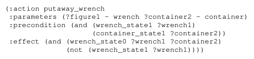
Finally, step 7 involves translating the complete FSMs into action models. The parameters and effects can be extracted from the state changes the corresponding transitions cause in the FSMs for each object sort. The bound state parameters added in steps 3-5 give the correlations between the action parameters and state parameters.

In our MACQ implementation, we first construct LearnedAction objects instead of outputting directly to PDDL. As MACQ didn’t previously have support for lifted action models, this step required the most overhead work to integrate. Classes for LearnedLiftedFluent and LearnedLiftedAction had to be added, as well as the tarski-powered “to PDDL” functionality.

The algorithm to perform step 7 was not provided. Instead, the authors pointed to another paper ( Citation: Simpson, Kitchin & al., 2007 Simpson, R., Kitchin, D. & McCluskey, T. (2007). Planning domain definition using GIPO. The Knowledge Engineering Review. Retrieved from http://eprints.hud.ac.uk/id/eprint/495/1/McCluskeyPlanning.pdf ) (some of their previous work) that uses a similar algorithm to translate FSMs to action schema. Despite some inconsistencies, we were able to reproduce the algorithm by referencing ( Citation: Simpson, Kitchin & al., 2007 Simpson, R., Kitchin, D. & McCluskey, T. (2007). Planning domain definition using GIPO. The Knowledge Engineering Review. Retrieved from http://eprints.hud.ac.uk/id/eprint/495/1/McCluskeyPlanning.pdf ) and iterating over the provided example.

for (sort, aps), states in zip(ap_state_pointers.items(), OS.values()):
    for ap, pointers in aps.items():
        start_state, end_state = LOCM._pointer_to_set(
            states, pointers.start, pointers.end
        )

        # preconditions += fluent for origin state
        start_fluent_temp = fluents[sort][start_state]

        bound_param_inds = []

        # for each bindings on the start state (if there are any)
        # then add each binding.hypothesis.l_
        if sort in bindings and start_state in bindings[sort]:
            bound_param_inds = [
                b.hypothesis.l_ - 1 for b in bindings[sort][start_state]
            ]

        start_fluent = LearnedLiftedFluent(
            start_fluent_temp.name,
            start_fluent_temp.param_sorts,
            [ap.pos - 1] + bound_param_inds,
        )
        fluents[sort][start_state] = start_fluent
        actions[ap.action.name].update_precond(start_fluent)

        if start_state != end_state:
            # del += fluent for origin state
            actions[ap.action.name].update_delete(start_fluent)

            # add += fluent for destination state
            end_fluent_temp = fluents[sort][end_state]
            bound_param_inds = []
            if sort in bindings and end_state in bindings[sort]:
                bound_param_inds = [
                    b.hypothesis.l_ - 1 for b in bindings[sort][end_state]
                ]
            end_fluent = LearnedLiftedFluent(
                end_fluent_temp.name,
                end_fluent_temp.param_sorts,
                [ap.pos - 1] + bound_param_inds,
            )
            fluents[sort][end_state] = end_fluent
            actions[ap.action.name].update_add(end_fluent)

fluents = set(fluent for sort in fluents.values() for fluent in sort.values())
actions = set(actions.values())

def to_pddl_lifted(
    self,
    domain_name: str,
    problem_name: str,
    domain_filename: str,
    problem_filename: str,
):
    """Dumps a Model with typed lifted actions & fluents to PDDL files.

    Args:
        domain_name (str):
            The name of the domain to be generated.
        problem_name (str):
            The name of the problem to be generated.
        domain_filename (str):
            The name of the domain file to be generated.
        problem_filename (str):
            The name of the problem file to be generated.
    """
    self.fluents: Set[LearnedLiftedFluent]
    self.actions: Set[LearnedLiftedAction]

    lang = tarski.language(domain_name)
    problem = tarski.fstrips.create_fstrips_problem(
        domain_name=domain_name, problem_name=problem_name, language=lang
    )
    sorts = set()

    if self.fluents:
        for f in self.fluents:
            for sort in f.param_sorts:
                if sort not in sorts:
                    lang.sort(sort)
                    sorts.add(sort)

            lang.predicate(f.name, *f.param_sorts)

    if self.actions:
        for a in self.actions:
            vars = [lang.variable(f"x{i}", s) for i, s in enumerate(a.param_sorts)]

            if len(a.precond) == 1:
                precond = lang.get(list(a.precond)[0].name)(*[vars[i] for i in a.precond[0].param_act_inds])
            else:
                precond = CompoundFormula(
                    Connective.And,
                    [
                        lang.get(f.name)(*[vars[i] for i in f.param_act_inds])
                        for f in a.precond
                    ],
                )

            adds = [lang.get(f.name)(*[vars[i] for i in f.param_act_inds]) for f in a.add]
            dels = [lang.get(f.name)(*[vars[i] for i in f.param_act_inds]) for f in a.delete]
            effects = [fs.AddEffect(e) for e in adds] + [fs.DelEffect(e) for e in dels]

            problem.action(
                a.name,
                parameters=vars,
                precondition=precond,
                effects=effects,
            )

    problem.init = tarski.model.create(lang)
    problem.goal = land()
    writer = iofs.FstripsWriter(problem)
    writer.write(domain_filename, problem_filename)

LOCM 2

LOCM2 is the successor to LOCM and makes a small but impactful change to the original algorithm. The original LOCM utilizes a sort-centered view of the domain, where a single state machine is defined for each sort. The issue with this is that certain domains contain objects which allow different behaviour for objects of the same sort depending on the internal state of the object. In LOCM this manifests itself as an output of overly permissive state machines. For instance in driverlog, the sort ‘truck' produces only a single state, which does not accurately map to its behaviour. “It should not be possible to perform two consecutive board_truck actions” and similarly a truck should only be able to drive when there is a driver present, hinting at the need for more than one state machine– one with and without a driver.

To address this, LOCM2 uses a different representation where each object is represented by multiple state-machines. LOCM2 uses transition-centered representation. States in the FSMs represent transitions which can affect the state of objects within a particular sort. Using the consecutive actions for each sort, the transition-connection matrix is defined and filled with holes. This matrix tracks which transition pairs change the states of the objects. Holes represent inconsistencies with which sorts are affected by consecutive actions. Using search to find the smallest set (which represents a state machine) which contains a hole and has a valid transition-connection matrix (all rows unique or non overlapping) LOCM2 records the auxiliary behaviour.

Results and Evaluation

To track our progression and validate our steps we constructed a test suite that tests the steps against the examples in the paper, and the algorithm in its entirety on the gripper domain. Our implementation passes all of the tests from the paper, producing the same output for each of the provided examples.

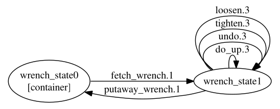
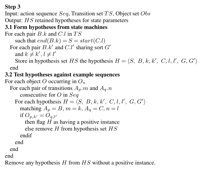
Step 1 uses a simplified tyre world action sequence as an example, and shows the following state machine as expected output.

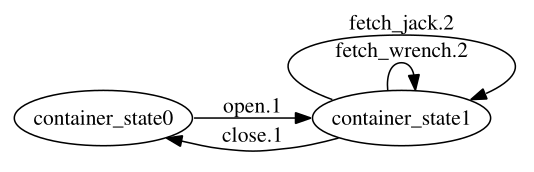
The generated output from our implementation is identical (apart from a different orientation and state naming, since object names are dropped in the actual algorithm).

Step 3 uses a different example action sequence, also from the tyre world domain, and states that in the sequence a hypothesis for $B.k=\text{putaway_jack}.1$, $C.l=\text{fetch_jack}.1$, and $k'=l'=2$ should be added and retained after filtering. Accordingly, our implementation builds this same hypothesis and retains it after filtering.

HS:
defaultdict(<function Hypothesis.from_dict.<locals>.<lambda> at 0x7faf703557e0>,
            {1: defaultdict(<class 'set'>,
                            {1: {<
  S=1
  B={'action': putaway_jack jack j2 container c2, 'pos': 2, 'sort': 1}
  k=2
  k_=1
  C={'action': fetch_jack jack j2 container c2, 'pos': 2, 'sort': 1}
  l=2
  l_=1
  G=1
  G_=2
>}}),
             2: defaultdict(<class 'set'>,
                            {1: {<
  S=1
  B={'action': putaway_jack jack j1 container c1, 'pos': 1, 'sort': 2}
  k=1
  k_=2
  C={'action': fetch_jack jack j1 container c1, 'pos': 1, 'sort': 2}
  l=1
  l_=2
  G=2
  G_=1
>}})})

Step 4’s example gives a hypothetical scenario with four hypotheses on a single state, then says that after running the step all of the hypotheses should be bound to the same variable. I.e. $v_1=v_2=v_3=v_4$.

bindings:

G=1, S=1
<
  S=1
  B={'action': loosen nut nut1 hub hub1, 'pos': 1, 'sort': 1}
  k=1
  k_=2
  C={'action': undo nut nut1 hub hub1, 'pos': 1, 'sort': 1}
  l=1
  l_=2
  G=1
  G_=2
> -> 0

<
  S=1
  B={'action': do_up nut nut1 hub hub1, 'pos': 1, 'sort': 1}
  k=1
  k_=2
  C={'action': tighten nut nut1 hub hub1, 'pos': 1, 'sort': 1}
  l=1
  l_=2
  G=1
  G_=2
> -> 0

<
  S=1
  B={'action': do_up nut nut1 hub hub1, 'pos': 1, 'sort': 1}
  k=1
  k_=2
  C={'action': undo nut nut1 hub hub1, 'pos': 1, 'sort': 1}
  l=1
  l_=2
  G=1
  G_=2
> -> 0

<
  S=1
  B={'action': loosen nut nut1 hub hub1, 'pos': 1, 'sort': 1}
  k=1
  k_=2
  C={'action': tighten nut nut1 hub hub1, 'pos': 1, 'sort': 1}
  l=1
  l_=2
  G=1
  G_=2
> -> 0

Finally, step 5 is the last step with a concretely presented, reproducible example. This one presents another bespoke FSM with four transitions, and concerns itself with a parameter on the state which is not referenced by one of the incoming transitions ($\text{jack_up}.2$). Therefore the parameter is flawed and should be removed, and our implementation does the same.

bindings:

G=2, S=1
<
  S=1
  B={'action': jack_up jack jack1 hub hub1, 'pos': 2, 'sort': 2}
  k=2
  k_=1
  C={'action': jack_down jack jack1 hub hub1, 'pos': 2, 'sort': 2}
  l=2
  l_=1
  G=2
  G_=3
> -> 0

<
  S=1
  B={'action': do_up nut nut1 hub hub1, 'pos': 2, 'sort': 2}
  k=2
  k_=1
  C={'action': undo nut nut1 hub hub1, 'pos': 2, 'sort': 2}
  l=2
  l_=1
  G=2
  G_=1
> -> 1


bindings after:

For step 7 and the results section of the paper, we were unfortunately unable to reproduce the exact same results as they used outdated or custom domains and the overhead in manually recreating these domains was unfeasible with our time constraints. Instead, we tested on the readily accessible domains (also conveniently built into MACQ) from planning.domains.

While LOCM is inherently incompatible with some of these domains (as discussed in the limitations in the original paper), it performed very well on the gripper domain. In this domain, there are multiple balls in different rooms, and two grippers can pick up and drop balls, and move between the rooms. Below are the complete FSMs learned for the domain, and the generated PDDL.

Ball sort FSM

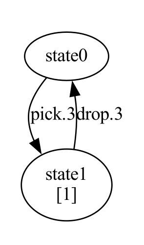
Gripper sort FSM

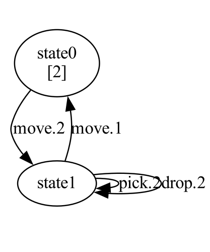
Room sort FSM

(define (domain locm)
    (:requirements :typing)
    (:types
        sort1 - object
        sort3 - object
        sort2 - object
        object
    )

    (:constants

    )

    (:predicates
        (sort1_state1 ?x1 - sort1 ?x2 - sort3)
        (sort1_state0 ?x1 - sort1 ?x2 - sort2)
        (sort2_state1 ?x1 - sort2)
        (sort3_state1 ?x1 - sort3 ?x2 - sort1)
        (sort2_state0 ?x1 - sort2 ?x2 - sort2)
        (sort3_state0 ?x1 - sort3)
    )

    (:functions

    )




    (:action move
     :parameters (?x0 - sort2 ?x1 - sort2)
     :precondition (and (sort2_state0 ?x1 ?x0) (sort2_state1 ?x0))
     :effect (and
        (sort2_state0 ?x0 ?x0)
        (sort2_state1 ?x1)
        (not (sort2_state0 ?x1 ?x0))
        (not (sort2_state1 ?x0)))
    )


    (:action pick
     :parameters (?x0 - sort1 ?x1 - sort2 ?x2 - sort3)
     :precondition (and (sort1_state0 ?x0 ?x1) (sort2_state1 ?x1) (sort3_state0 ?x2))
     :effect (and
        (sort3_state1 ?x2 ?x0)
        (sort1_state1 ?x0 ?x2)
        (not (sort1_state0 ?x0 ?x1))
        (not (sort3_state0 ?x2)))
    )


    (:action drop
     :parameters (?x0 - sort1 ?x1 - sort2 ?x2 - sort3)
     :precondition (and (sort3_state1 ?x2 ?x0) (sort2_state1 ?x1) (sort1_state1 ?x0 ?x2))
     :effect (and
        (sort1_state0 ?x0 ?x1)
        (sort3_state0 ?x2)
        (not (sort3_state1 ?x2 ?x0))
        (not (sort1_state1 ?x0 ?x2)))
    )

)

References