Continuous Authentication

Participants

Jagrit Rai

This project aims to build a process to allow for continuous authentication on a computer terminal using users typing characteristics acquired from sensor data from a smartwatch worn by the user while typing. This method of authentication is useful when multiple users have access to a single PC, whether by permission of the owner of the machine or due to the owner leaving a computer unattended in a crowded environment.

Our objective

We aim to create a system architecture that can allow for seamless continous authentication for users in an office environment, which can accurately identify attackers and verify users in a non-intrusive manner.

System Pipeline

Overview

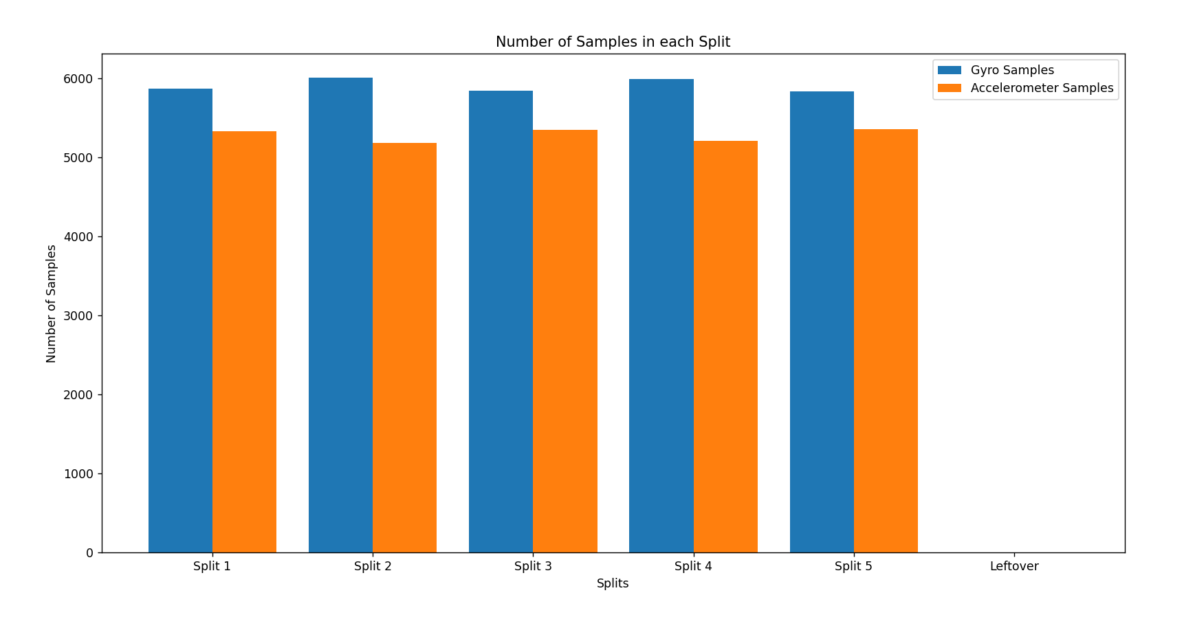
Data collected from a user is loaded into a large general dataframe. This dataframe is split into 5 chunks. These chunks are then seperated into two separate dataframes based on the type of sensor the data belongs to.
Data from these chunks then run through preprocessing, which returns a list of dataframes that contain filtered axis data from both sensors.
Each of the these filtered dataframes then pass through the feature extraction process, which then returns a list of feature vectors.
These vectors are all then labelled with the user ID.
This process is completed over all users in the system to compile a database of all user feature vectors. For Test 1 data, this database is used as training and testing for a classifier module to differentiate between different users based on new feature vectors.

User Data Collection

Data is collected from users from a series of tests. Test 1 consists of all users typing the same text. This test is used as registration data for all users. Users wear a smartwatch on their wrist as they type, which collects gyroscope and accelormeter data across 3 axes.

Preprocessing

A row of raw data appears as row $r = {t, x_s, y_s, z_s}$ where $t$ is a timestamp, and $x,y,z \in S$ where S is a sensor, either gyroscope or accelerometer.
In the preprocessing step, we apply an M-point Moving Average Filter to the raw data in order to reduce the impacts of noise on feature data. In our experiments, we have set M = 9.
We then set a window size $N$ to define how many samples are used to calculate a single feature vector. In our experiments, we found success with sample sizes of $N = 1500$. If the frequency of the sensor is 100hz, 1500 samples is equivalent to 15 seconds of typing data.
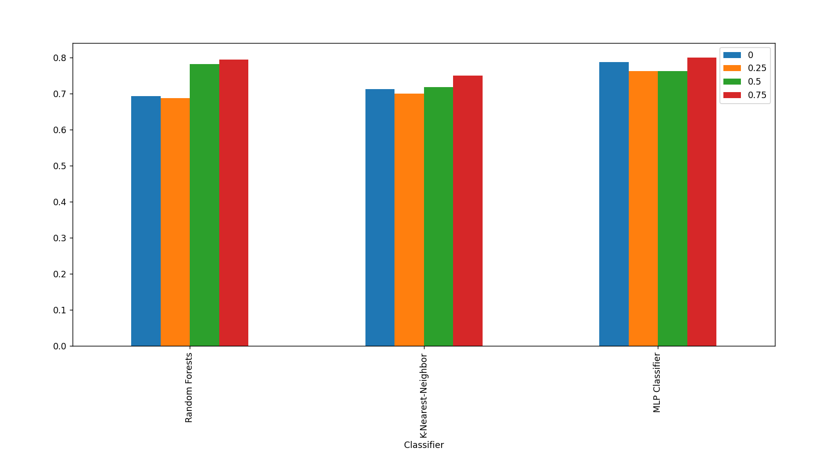
These windows can be overlapped with each other at various intervals. This works by having each window begin on a row included in the previous window, allowing for windows to include data from prior windows. The reason for this inclusion was to account for rough cutoffs in datastreams that may occur if no overlap is included; for example, short keystrokes not being analyzed in their entirety, becoming obscured by longer periods of trailing idleness. In our experiments, we worked with overlapping these by 0%, 25%, 50% and 75%.
After overlapping windows and filtering data, each single sample of gyroscope and accelerometer data is placed into a single row, shedding their timestamps. Thus, a row of data now occurs as row $r = {x_a, y_a, z_a, x_g, y_g, z_g}$.

Feature Extraction

Features are calculated and extracted from each column on dataframes produced from the preprocessing step. Features calculated include features in the domain of time, and features in the domain of frequency. The features we calculate are
Mean, Median, Variance, Average Absolute Difference of Peaks, Range, Mode, Covariance, Mean Absolute Deviation, Kurtosis, Skewness, correlation between axes (xy, yz,xz), Minimum, Maximum, Root Mean Square, Entropy, Spectral Energy
These 17 features extracted over 6 columns results in a total of a feature vector of length 102. Feature vectors are calculated upon each window. The vector normalized before being returned.

User Profiling

Feature vectors are labelled by user ID.
A user profile is created, of the form $ p = <userID, time_{start}, time_{end}, \vec{registrationData}, \vec{featureData}>$ where $\vec{registrationData}$ is the collection of all feature vectors calculated from test1, and $\vec{featureData}$ is the collection of all other calculated feature vectors from any other test

Classificatons

Labelled feature vectors from user registration data are compiled into a database
This data is then fed into a classifier; we tested with MLP, Random Forests and K-Nearest-Neighbour
Data is split using a 5-fold cross validation method, such that for each fold, 80% of the data is used as training data and 20% is tested upon. Naturally, a different 20% is tested on with the remaining data used for training each split.
Average accuracy of all 5 splits are calculated and used in graph data

Problems Faced

A point of confusion was somewhat inconsistent raw user data. For example, the frequency of accelerometer and gyroscope data was uneven. This caused a general lack of data to work with, as well as an overrepresentation of gyroscope data, resulting in accelerometer data to not be considered as heavily in our classifiers. Another issue this caused was that datapoints were often not aligned properly, causing data from the underrepresented sensor to be present in the wrong chronological windows. This was due to our initial method of separating chronological windows by number of samples. For example, if there are 10 total samples of accelerometer data and 100 samples of gyroscope data collected over 100 seconds, a window of the first 10 seconds would contain 10 seconds worth of gyroscope data, but the entire 100 seconds worth of accelerometer data.
Classifier issues. Note that initially results were topped out around 20%

2a. Part of the issues was uneven weighting of data, could have 17 samples of user1 data compared to 12 samples of user19 data vs 10 samples of user47 data

2b. Data was all layered on top of each other in order; what this caused was for certain users to never be counted in different splits. For example, in split 1, users are used as train data, while the bottom 20% would be test data. However, when data is ordered by user, what this means is that the bottom 20% will consist of users whose data has never been trained upon.

2c. The low the number of samples per user, the worse the classifier performs. This is quite obvious, however the original WACA paper reported high accuracies with 5 samples per user. This was not the case in our experiments. In order to achieve higher accuracy results, we used 10 samples per user.

Solutions

The makeshift solution we worked with was to simply throw out user data that had a great disparity between sensor data. However, we have moved on to exploring a more comprehensive solution by separating chronological windows by actual length of time, rather than separating number of samples based solely on taking for granted the sampling frequency.
Solutions to Classifier Issues

a. We solved the uneven weighting of data by passing a parameter to specify a uniform amount of samples per user. There are downsides to this solution– If a user does not have enough samples to meet this parameter, their data simply is not included in the training/testing data. If a user has more than enough samples, their surplus data is not considered.

b. User samples were arranged such that exactly one sample comes from every user until all have been represented, at which point we once again place one row of data from each user, until all data has been used. Ordering data in this way ensures that no user is ever completely absent from training or testing splits.

c. The low number of user samples was tackled by overlapping windows of raw user data. By doing this, we are able to make the most of the collected data and extract more feature vectors per user.

Our Modifications

Overlapping of user windows
- Sensor axis data was split into windows of variable sizes; features are then extracted from these windows. A window of 1500 samples would be equivalent to 15 seconds (1500 samples at a sampling frequency of 100hz) of typing data. In our implementation, we experiment with overlapping the data from these windows by 25%, 50% and 75% to compare the effects on accuracy. Not only does this overlap provide us with more extracted user data, it also helps to account for the loss of information when windows abrubtly cut off information streams, such as when a window captures only half of a keystroke.
Running splits pre compression
Preservation of time-series integrity; splitting based on time rather than number of samples.
This ensures that if for whatever reason the sampling rate of the sensors is not 100hz as reported, there will be no issues of unintended overlaps of data.