Football Field Perspective Shift

Abstract

Sports Analysis is a project where a user inputs a video clip of an American football game, it detects the lines on the pitch and visualizes the output overlaid on the original video. It consists of two parts: one uses a computer vision library such as OpenCV to detect the lines on the field on the image, and one corresponds the points on the image to the blueprint. The module of detect_lines uses openCV and cv2 to detect lines on the pitch, and we further optimize the results by dividing all the lines into three categories: vertical, horizontal, and oblique lines. Then optimize the classification within the group by establishing different distance thresholds and slopes specifically to the oblique lines. For the second part of the project, mapping any point in the input image to the 2d blueprint is a mathematical translation between the real-time frame of the video and the given football field. The main concept is that we allow for the manual specification of 3-4 points in the frame and their matching 3-4 points in the blueprint to form a quadrangle. From those manually given coordinate pairs, make the hover work from frame-to-blueprint and blueprint-to-frame. Finally, we applied streamlit to make it an interactive web page with users who can upload videos and modify parameters to get the video effect they want. It would be beneficial for football players to evaluate their teammates' performance during games, which would aid in the post-game analysis and assist coaches to better their strategies and training regimens.

Introduction

Sports analytics is the analysis of sports data, including components of sports such as player performance, business operations, and recruitment. The data offers an advantage to both individuals and teams participating in a competition and sports enterprises. Sports analytics uses the application of mathematical and statistical rules to sports. On-field analytics enhance the performance of players and coaching staff by focusing on their strategies and fitness.

Data analysis helps sports entities evaluate the performance of their athletes and assess the recruitment necessary to improve the team performance. It also evaluates the strong and weak areas of their challenger, enabling coaches to make the right decision on their tactics. ( Citation: Indeed Editorial Team, nd Indeed Editorial Team (nd). What Is Sports Analytics? (Definition, Importance, and Tips). Retrieved from https://ca.indeed.com/career-advice/finding-a-job/what-is-sports-analytics#:~:text=Sports%20analytics%20is%20the%20analysis,a%20competition%20and%20sports%20enterprises. )

Background

This open-ended project is for focusing on advanced sports analytics. The goal of this project is to detect lines in the fields and create visualizations from a given American football game video, to determine team influence of player behavior, etc.

It’s all kind of trivial if you have a top-down view (already 2d), and even fairly easy if the camera is stationary. But those are very rare circumstances. Camera is usually focusing on the players who hold the ball, and the situation is complicated during the match, this project aims to detect lines in each frame as the camera moves around. Since there’s already work underway that should identify players. If we ignore players in the football field, there should be more fun stuff down the line to explore.

The project is mainly divided into two parts. First part is given an image or video about American football, the program would identify the lines in the field. Second part is to find where the image is pointing compared to a known blueprint (top-down view of the football field) so that any point in the image can be mapped to the 2d coordinates. These two parts can be done concurrently (even if it seems like 2 depends on 1), and both are essential components in the larger pipeline of sports analytics.

Approach

First and foremost, we need to determine the image recognition method used to identify the lines on the football field. After researching, we chose OpenCV, an open-source computer vision library. It implements many common algorithms in image processing, and it brings benefits in human-computer interaction, computer vision, machine learning and other related algorithms.

Preprocessing

We installed OpenCV and started our journey to detect lines of football fields. To begin, we converted colored images to grayscale images with cvtColor(image, cv2.COLOR BGR2GRAY). Doing the transformation is because the information contained in color images is too large, and when performing image recognition, it is actually sufficient to use only the information in grayscale images, so the purpose of image graying is to improve the speed of computing. While the color information has been lost, the texture, lines, and contours have been preserved, which are typically more important than color features. Furthermore, the grayscale images may be improved by using bitWise_and(), which was used to regulate the channel or the output region by masking, making it easier to extract the image structural elements or modifying the pixel values in an image.

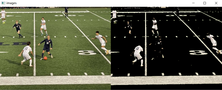
Then we found that there were still many outlier pixels that could be noise in the image, so we applied GaussianBlur(), a method of blurring the image, to the gray image. It uses a Gaussian kernel and the width and height of the kernel must be positive and odd. The Gaussian filtering is mainly used to eliminate Gaussian noise, which can retain more image details and is often referred to as the most useful filter.

Detect Lines in Fields

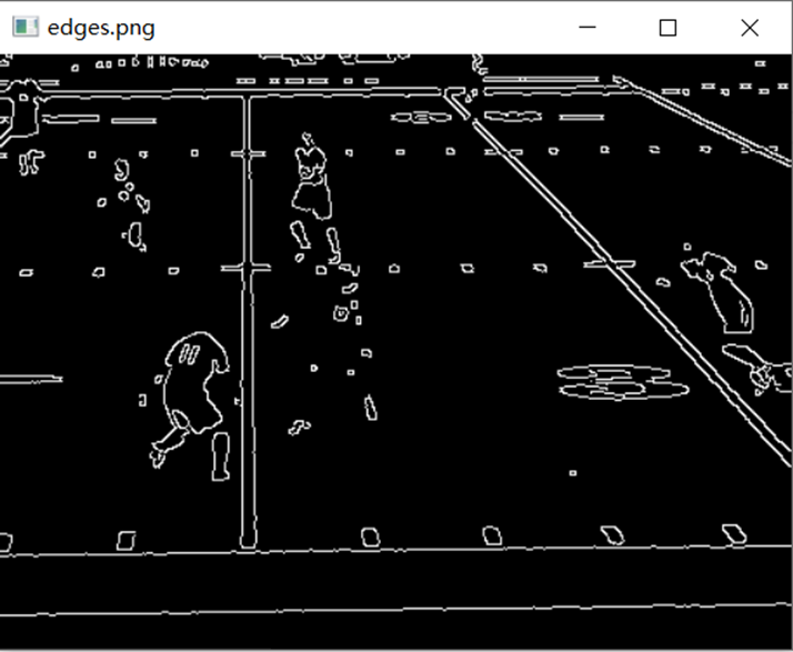
As the noise pixels were removed and the image became much smooth now, the picture preprocessing step was mostly done. Next, we came to the step that detect edges, which are features that can be used to estimate and analyze the structure of objects in an image and represent significant local changes that occur in the image intensity (i.e., pixel values). We used the Canny() method of the cv2 library to detect the edges in the image using the canny edge detection algorithm. The first thing it does is, it uses Gaussian convolution to smooth the input image and remove noise. Then, the first-order derivative operator is applied to the smoothed image to highlight image regions with high first-order spatial derivatives. To reassemble the broken parts of the object and expanding the highlight in the image, cv2.dilate() is used. It helps to apply morphological filters to photos and zoom in on foreground items.

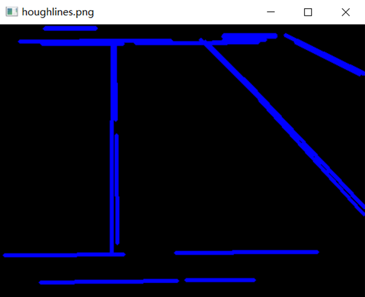
A method for finding line segments is the Hough line transformation. The basic principle of the Hough transform lies in using the duality of points and lines to change a given curve in the original image space into a point in the parameter space through the form of a curve expression. This transforms the detection problem of a given curve in the original image into a problem of finding a peak in the parameter space. That is, the detection of the overall characteristic is transformed into the detection of the local characteristic. We met the requirements for applying the Hough transformation after pre-processing edge detection. HoughLinesP() has a number of parameters, all of which have a significant impact on the final graph.

The function HoughLinesP() takes the following parameters.

• image: must be a binary image, recommended using the resulting image of canny edge detection.
• rho: the distance accuracy of the line segment in pixels, double type, 1.0 is recommended
• theta: the angular accuracy of the line segment in radians, numpy.pi/180 is recommended
• threshold: the threshold parameter of the accumulation plane, int type. It exceeds the set threshold before the line segment is detected. The larger the value, which basically means that the longer the detected line segment, the fewer the number of detected line segments. It is recommended to try with 100 according to the situation
• minLineLength: the minimum length of a line segment in pixels, set according to the situation
• maxLineGap: the maximum allowable interval between two line segments in the same direction as one line segment. If the value is exceeded, the two line segments will be treated as one line segment. The larger the value, the larger the break in the line segment is allowed, and the more likely to detect a potential straight line segment.

These parameters can greatly affect the line segments that can be recognized, especially the last three parameters. Each of the distinct images must be adjusted on a regular basis in order to achieve the best possible result. We tried several times and concluded some default values that can get relatively good results in general cases. ( Citation: Christopher Haywood, nd Christopher Haywood (nd). Detecting tennis court lines intercepts. Retrieved from https://stackoverflow.com/questions/55496402/detecting-tennis-court-lines-intercepts )

Optimization of Line Detection

After using OpenCV to draw Hough lines, we can have a stretch for the line detection. However, it might seem visual for human eyes, but not for the computer to discover its pattern behind line segments. Many line segments meant to be the same line are mixed very closely, some of them are intermittent, and others seem not to have the right slope. Some parallel line segments are only a few pixels away from others and they are considered as the different lines by OpenCV. To reduce redundant and distracting lines, we need to merge line segments.

What kind of line segments should be merged into one line? Based on the image observed, there were line segments that are broken in the middle or have very close slopes, that can be merged. As a result, the first thought that came to mind was to look for parallel lines or line segments that may be termed parallel. We need to calculate the slope, and the formula for the slope is k=(y2-y1)/(x2-x1) at two points (x1, y1) and (x2, y2). So we chose to traverse all the lines, write down their coordinates, and compute the slope. We soon found the issue: the slope of horizontal and vertical lines is either 0 or infinite. We determined to split the horizontal and vertical lines as this was not suitable for processing and dividing. This initially laid out the three sets of lines we needed to deal with: horizontal lines, vertical lines, and oblique lines.

To deal with the possible error when computing the k value, we opted to use x1-x2=0 to determine if the line is vertical and y1-y2=0 to determine whether the line is horizontal; the rest are all considered oblique lines. Following that, we can conduct various responses for various line sets.

It is worth mentioning that in order to add flexibility to the recognized images, we set thresholds as parameters. The distance thresholds are of vital importance since the identification of lines will be intermittent, and they affect which lines can be merged into one line. Therefore, if the threshold is set too large, two lines that are originally irrelevant or even far apart will be recognized as one line, but if the threshold is set too small, the two line segments that are originally the same straight line cannot be connected. Moreover, the threshold of k value also has a great influence on the result. It can determine whether the two oblique lines are parallel. Combined with the threshold of the k value and the distance threshold of oblique lines, we can group those with similar distances and similar slopes to determine whether they can be merged.

For vertical and horizontal lines, we decided to use extended lines. Within the threshold given, we first need to create three empty lists to collect data from parameters. The first list aims to store x coordinates for vertical lines and y coordinates for horizontal lines independently. The second list aims to reduce corresponding coordinates within the threshold. To be specific, we considered these lines as the same line if they are within the threshold and treat them as errors. Therefore, we only add every first coordinate that meets the condition to this list and then compare to find the next one. Then, we compared every line coming from the parameter with the second list. If the corresponding coordinate is within the threshold, we checked whether this line’s start point or end point is larger than the maximum value, or smaller than the minimum value. We first set the assumed maximum and minimum value before comparison and change it continuously during the loop if a new extreme point occurs. Finally, we added the merged lines into the third list. with fixed x coordinate as its new x coordinate in both start point and end point, minimum value as its start point’s y coordinate, maximum value as its end point’s y coordinate for vertical lines. Horizontal lines have the same algorithm when we exchange x and y coordinates.

For oblique lines, things were quite different. The method of extended line didn’t work well when it came to oblique lines. Our mathematical idea changed to calculate the shortest distance between the start point and other lines extended long enough. In order to achieve this, we created two lists containing the first line as the base line. The line segments in the line set passed in have the similar slope (k value). We compared the first line to every other lines’ start point to calculate their distance using get_distance() which returns the distance between the given point and line using the mathematical formula. If the distance is within the threshold and compared to the second list, we create it to check whether it has been compared before, if not, add the compared line into two lists, first one to store the matching lines within the loop, while second to store lines globally for comparison. After having the matching lines’ list, we just need to find the four extreme value in the list, x_min, x_max, y_min, y_max using find_extreme() which is used to compare every x and y coordinate and returns the maximum and minimum value, and clean the first list to make it ready for the next loop. By double checking the k value again to enhance its reliability and calculate whether the k value is positive and negative, we were able to create the corresponding merged line in this loop.

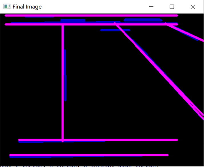
Image Translation

For the second part of the project, we need to map any point in the input image to the 2d coordinates, also called blueprint. It is the mathematical translation between the real-time frame of the video and the given football field, which allows sports analysts to see how each player responds under the circumstance from the top-down 2d blueprint view. The main concept of this part is that we assume that the anchor points are given, which are four vertices of the field forming a quadrangle. We allow for the manual specification of 3-4 points in the frame and their matching 3-4 points in the blueprint. From those manually given coordinate pairs, make the hover work from frame-to-blueprint and blueprint-to-frame. In the beginning, we set the mouse handler for the images and called the click event functions using cv2.setMouseCallback() from OpenCV to record the mouse events for both the blueprint and the frame. The click event functions are different between frame-to-blueprint and blueprint-to-frame, the concepts of translation process are similar, but there is some small difference when transform rectangle into quadrangle (blueprint-to-frame).

For the frame-to-blueprint click event, if we click any point in the frame using the mouse, the cv2.setMouseCallback() will tell us the x and y coordinates where we clicked. We use the get_distance() function from the previous part to calculate the distance between the clicked point and each boundary line generated by the anchor points we assumed. Next, we shift the x coordinate of the initial top-left blueprint anchor point to the right, with the horizontal line’s length times the proportion of the distance from the clicked point to the left and right boundary calculated above. Then we shift the y coordinate of the anchor point down, with the vertical line’s length times the proportion of the distance from the clicked point to the top and down boundary. Finally, we display the mapped coordinates in the blueprint, and we are done.

For the blueprint-to-frame click event, it is a little more difficult than before. The method is similar, we first calculate the distance between the clicked point and each boundary line generated by anchor points we assumed in the blueprint. Next step is the most important concept in the process, we shift the frame coordinate given by the proportion of the distance from the clicked point to the boundary, using the similarity property of triangular and then find the well-proportioned point in each boundary line. Take the top boundary as the example, we calculate the distance from clicked point to the left boundary and the entire length of top boundary line in the blueprint, its proportion should be exactly the same proportion in the frame for the same boundary, so we shift the top-left corner anchor point in the frame to the right and down with this proportion since the proportion in hypotenuse (the given frame boundary) should be the same when it comes to legs (x and y coordinates). After getting four well-proportioned points, we check the intersection of these points to locate the mapped coordinates that we want using the mathematical approach in Euclidean geometry. ( Citation: Wikipedia, nd Wikipedia (nd). Line–line intersection. Retrieved from https://en.wikipedia.org/wiki/Line%E2%80%93line_intersection ) We have already written the approach as a function so it can be used any time. Finally, we display the mapped coordinates in the frame when we click some point in the blueprint.

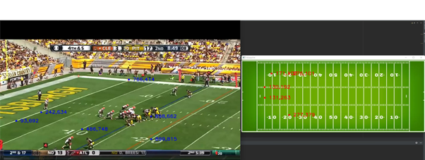
As a result, if the customers click any point in the frame, they should get the corresponding location in the blueprint with red color showing its coordinates and exact location with an asterisk. If the customers click any point in the blueprint, they should get the corresponding location in the frame with blue color showing its coordinates and exact location with an asterisk as well. They can close both the window of the frame and the blueprint to end the program.

Evaluation

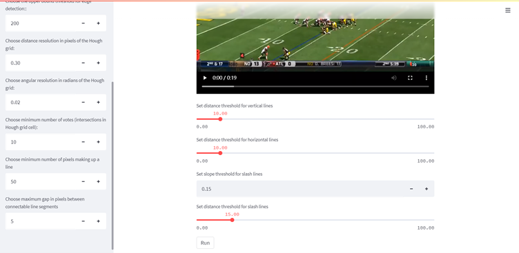
Now our function can do a pretty accurate identification of the lines on a football field image, next we just need to split the video into dozens of images based on the number of frames, do the identification and then combine the identified images into a new video. At the suggestion of our mentor, we learned that we could use streamlit to create a demo URL. So, we tried to link the written back-end processing with the front-end web page, allowing users to upload their own videos and adjust the parameters for pitch line recognition. To wrap up, all we need from the user is the file to be recognized (in MP4 format), and a few relevant parameters that have default values and could be changed by the user.

We have divided streamlit into three sections.

• Sidebar: It contains 8 parameters that are closely related to the drawing. They are mainly applied to steps such as detecting line segments, Hough transformations and determining the number and quality of identified line segments.
• Main part: This part contains the video that needs to be uploaded by the user, and four other parameters closely related to the line segment optimization. They are mainly used to optimize the identified line segments, such as optimizing the breakpoints between line segments and merging broken line segments together.
• Output part: after uploading the video and adjusting the parameters, click the run button to wait for the video to be generated. It takes a few moments to generate the video for the test video, and the detected lines will be overlaid on the original video clearly. The output video will appear on the website for a preview.

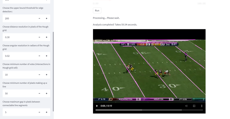
The output video looks like this, it shares the same resolution and frames per second as the input video, with merged field lines highlighted.

Summary

This project successfully detects lines in the fields and creates visualizations from a given American football game video, to determine team influence of player behavior, etc. Most of the field lines can be identified correctly even across the players, except for the auditorium and the blurred places as the camera moving that cannot be accurately identified.

Due to the time limit, we started the term assuming this could be aligned automatically, but to simplify, we now assume we have some reference points (anchor points). In future, the automatic alignment will be done, and the project will do the location translation between every frame in the video and the given blueprint without any manual specification.

Additionally, there is an optimized approach for the blueprint-to-frame part, we assume we have a parallelogram by now to calculate the proportion. However, this is not always the case, since the view of the camera is shifting, and the field tend to be the trapezoid rather than parallelogram. As the result, part of the mapping translation right now is not very accurate. We could find the opposite lines that are not parallel in the frame, find the proportion by distance from the blueprint, draw the perpendicular lines for those lines in the frame, and then find the intersection point. This approach should reduce the error for translation. I have not found a better mathematical solution for frame-to-blueprint part, but the problem facing is the same. We need to find a fit translation between the rectangle blueprint and any quadrangle frame.

References